Classifiers, table of contents
Discriminant is a classifier that directly separates the classes instead of modeling them. Providing only class distinction, discriminants cannot be used for detection.
- 13.1.1. Fisher linear discriminant
- 13.1.2. Least mean square classifier
- 13.1.2.1. Performing linear regression
- 13.1.3. Logistic classifier
- 13.1.3.1. Polynomial expansion
- 13.1.3.2. Optimization algorithm
13.1.1. Fisher linear discriminant ↩
Fisher discriminant sdfisher performs linear discriminant analysis
extraction (LDA) with sdlda to find an informative subspace where the
classes are well separated. The dimensionality of the resulting subspace is
typically the number of classes - 1.
In this subspace, sdfisher trains a linear classifier assuming normal
densities. In this way, we obtain a general solution that is applicable to
any number of classes.
The Fisher discriminant is very similar to liner discriminant assuming normal
densities sdlinear, although it does not use explicit assumption of
normality but only second order statistics.
To train a Fisher discriminant on a data set, use:
>> p=sdfisher(a)
sequential pipeline       2x1 'Fisher linear discriminant'
1 LDA                     2x2
2 Gaussian model          2x3  single cov.mat.
3 Normalization           3x3
4 Decision                3x1  weighting, 3 classes
13.1.1.1. Avoiding over-fitting of Fisher discriminant ↩
Although Fisher discriminant can be trained on problems with small number of samples and large number of features (even with more features than samples), this often yields over-training. The resulting classifier shows high performance on the training set but fails to generalize on the test set.
One way to avoid over-training is to consider dimensionality reduction using
sdpca to prepare a lower-dimensional subspace:
>> a
'medical D/ND' 6400 by 11 sddata, 3 classes: 'disease'(1495) 'no-disease'(4267) 'noise'(638)

>> p1=sdpca(a,0.9)
PCA pipeline              11x2  94% of variance
>> p2=sdfisher(a*p1)
sequential pipeline       2x1 'Fisher linear discriminant'
 1 LDA                     2x2
 2 Gaussian model          2x3  single cov.mat.
 3 Normalization           3x3
 4 Decision                3x1  weighting, 3 classes
The total pipeline is then composed of both PCA and Fisher classifier:
>> p=p1*p2
sequential pipeline       11x1 'PCA+Fisher linear discriminant'
 1 PCA                    11x2  94%% of variance
 2 LDA                     2x2
 3 Gaussian model          2x3  single cov.mat.
 4 Normalization           3x3
 5 Decision                3x1  weighting, 3 classes
13.1.2. Least mean square classifier ↩
The least-mean square classifier performs linear regression on numerical representation of class labels.
>> a
'Fruit set' 260 by 2 sddata, 3 classes: 'apple'(100) 'banana'(100) 'stone'(60)

>> p=sdlms(a)
sequential pipeline       2x1 'Least mean squares+Decision'
1 Least mean squares      2x3
2 Decision                3x1  weighting, 3 classes
By default, all classes bare identical weights in the internal regression task. We may want to change that if we have a prior knowledge that some of the classes are more important and related class errors are more costly. This may be achieved by the 'cost' option providing a numerical vector for per-class costs:
>> p2=sdlms(a,'cost',[0.1 0.8 0.1])
sequential pipeline       2x1 'Least mean squares+Decision'
 1 Least mean squares      2x3
 2 Decision                3x1  weighting, 3 classes
The p2 classifier considers 'banana' class more important than 'apple' or
'stone'.
13.1.2.1. Performing linear regression ↩
The sdlms may also be used to regress arbitrary user-defined numerical
targets. The soft outputs of sdlms then provide resulting linear
regression predictions.
>> a
'Fruit set' 2000 by 2 sddata, 3 classes: 'apple'(667) 'banana'(667) 'stone'(666)
>> [tr,ts]=randsubset(a,0.5);
>> T=-tr.lab;
On the last line, we create a numerical vector T with label indices (1,2,
and 3). We can use this as target definition for regression:
>> p3=sdlms(tr,'targets',T)
Least mean squares pipeline 2x1
Note that, when used for regression, sdlms does return soft outputs.
Applying the pipeline on test data yields predicted values:
>> ts([5:6 500:505])
'Fruit set' 8 by 2 sddata, 2 classes: 'apple'(2) 'banana'(6)
>> +ts([5:6 500:505])*p3

ans =

1.6542
1.8665
2.0208
1.4559
1.3640
1.0728
2.4711
2.2565
13.1.3. Logistic classifier ↩
sdlogistic implements a classifier based on logistic regression. By
default, it builds a single direct multi-class model which is non-linear
due to polynomial feature space expansion step.
>> a
'Fruit set' 260 by 2 sddata, 3 classes: 'apple'(100) 'banana'(100) 'stone'(60)

>> p=sdlogistic(a)
sequential pipeline       2x1 'Logistic classifier'
 1 Feature expansion       2x7
 2 Scaling                 7x7  standardization
 3 Logistic classifier     7x3  degree 3
 4 Decision                3x1  weighting, 3 classes
>> sdscatter(a,p)
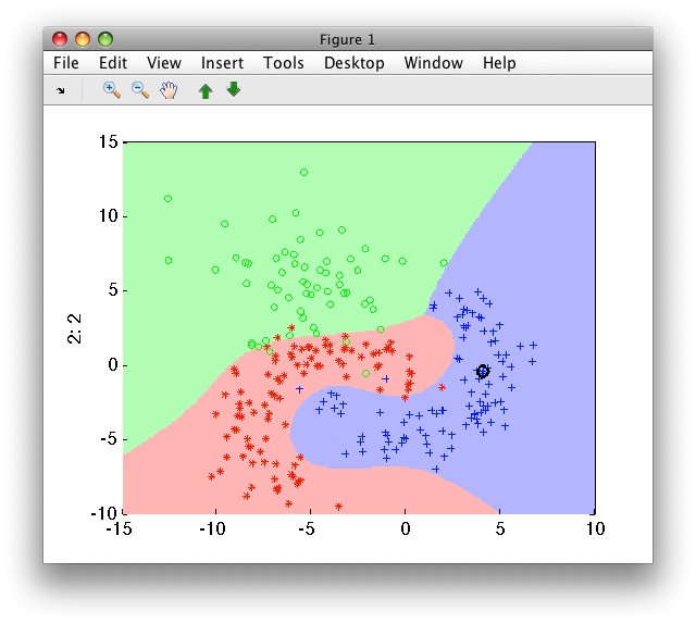
In the example above, the input 2D feature space is expanded using 3rd degree polynomial terms to 7D space. In this space, scaling is applied and logistic classifier is trained.
13.1.3.1. Polynomial expansion ↩
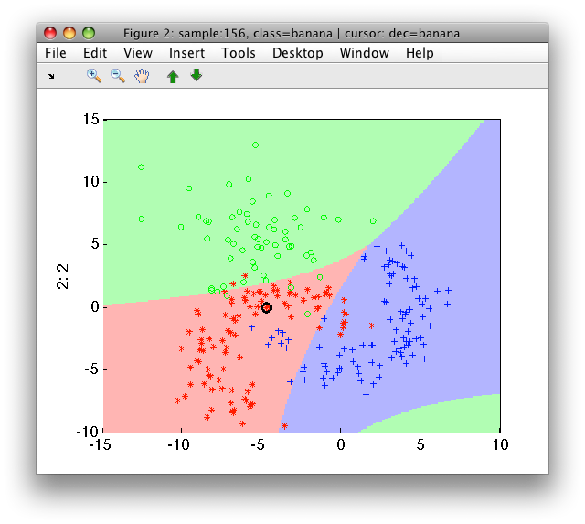
The polynomial expansion may be controlled using the 'degree' option. For example, using degree of 2 may not be sufficient for the fruit problem, which requires cubic decision boundary:
>> p2=sdlogistic(a,'degree',2)
sequential pipeline       2x1 'Logistic classifier'
 1 Feature expansion       2x5
 2 Scaling                 5x5  standardization
 3 Logistic classifier     5x3  degree 2
 4 Decision                3x1  weighting, 3 classes
>> sdscatter(a,p2)
Polynomial expansion is handled by sdexpand command. If you prepare the
desired feature space manually, you may disable expansion in the
sdlogistic with 'no expand' option:
>> a
'Fruit set' 260 by 2 sddata, 3 classes: 'apple'(100) 'banana'(100) 'stone'(60)
>> ppoly=sdexpand(a,5)
Feature expansion pipeline 2x11
>> ppoly.lab'
   1 F1:1
   2 F2:2
   3 F1^2
   4 F2^2
   5 F1^3
   6 F2^3
   7 F1^4
   8 F2^4
   9 F1^5
  10 F2^5
  11 F1*F2
>> b=a*ppoly
'Fruit set' 260 by 11 sddata, 3 classes: 'apple'(100) 'banana'(100) 'stone'(60)

>> p3=sdlogistic(b,'no expand')
sequential pipeline       11x1 'Logistic classifier'
 1 Scaling                11x11 standardization
 2 Logistic classifier    11x3  degree 3
 3 Decision                3x1  weighting, 3 classes
13.1.3.2. Optimization algorithm ↩
Optimization of the logistic classifier is performed using gradient descent algorithm. It may be influenced by changing number of iterations and optimization step.
The number of iterations is changed by 'iters' option. By default, 10000 iterations are performed.
The step can be altered by 'step' option. The default step value is
0.01. Using larger step values, we be find the same solution
faster. However, the danger is that we are too fast and diverge from the
optimal solution. In such case, sdlogistic raises an error suggesting to
use smaller step:
>> p4=sdlogistic(a,'step',0.2)
{??? Error using ==> sdlogistic at 144
Optimization failed (NaN or infinite value detected). Try to adjust the
optimization 'step' value (typically make it smaller). You may also check the
progression of likelihood in the second output param - example:
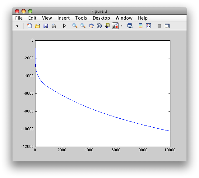
[p,res]=sdlogistic(data,'step',0.001); figure; plot(res.L)
The progress of optimization may be visualized by plotting the likelihood
value. It is returned in the optional second output res:
>> [p5,res]=sdlogistic(a)
sequential pipeline       2x1 'Logistic classifier'
 1 Feature expansion       2x7
 2 Scaling                 7x7  standardization
 3 Logistic classifier     7x3  degree 3
 4 Decision                3x1  weighting, 3 classes

res =

degree: 3
  step: 0.0100
     L: [10000x1 double]

>> figure; plot(res.L)
The plot shows log-likelihood development over the 10000 iterations. The lower the value the better fit of the model to data.