This chapter describes how to identify clusters in the data using unsupervised cluster analysis methods.
- 18.1. Introduction
- 18.2. Clustering with sdcluster command
- 18.2.1. Clustering all data irrespective of classes
- 18.2.2. How to cluster already clustered data set?
- 18.2.3. Changing default cluster names
- 18.2.4. Removing cluster labels
- 18.3. Clustering algorithms
- 18.3.1. k-means algorithm
- 18.3.1.1. Obtaining cluster labels with sdkmeans
- 18.3.1.2. Accessing prototypes derived by sdkmeans
- 18.3.2. k-centers algorithm
- 18.3.3. Gaussian mixture model
18.1. Introduction ↩
Cluster analysis, also called unsupervised learning, groups similar observations into clusters. In this way, we may learn what typical situations occur in our data set. Cluster analysis aims at answering questions such as:
- Is there structure in my data?
- What are typical clusters/groups are in this data set?
There are two typical uses of cluster analysis. The first one aims at interpretation of clustering result. For example, we cluster an image (set of pixels in RGB feature space) and obtain a set of 10 clusters that represent different image regions. We then interpret (give meaning) to some of these clusters. In this way, we identify that some clusters represent sky, buildings or trees. With these new labels, we may train a specific classifiers applicable to new images.
Secondly, cluster analysis is often adopted as a tool for building a flexible data representation in complex supervised problems. The resulting set of clusters is used, for example, as prototypes for building better classifiers in multi-modal problems.
With perClass, you may quickly cluster even very large data sets, easily interpret the results, and directly leverage this information for building your classifiers.
18.1.1. Example of using cluster analysis to build a pixel classifier ↩
Say we want to detect road in images. However, all we have are images without road labels. Instead of painting the road region by hand, we will use clustering to define class labels.
First, we will load the image:
>> im=sdimage('roadsign18.bmp','sddata')
412160 by 3 sddata, class: 'unknown'
and visualize it:
>> sdimage(im)
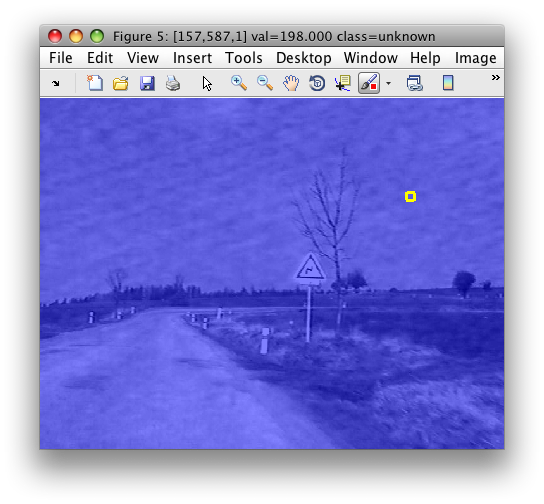
The image shows a scene captured from a car. Note that we started from an image without any label information. Therefore, the image data set contains only the 'unknown' class.
We will now use cluster analysis to find clusters in this data set. We use
the high-level sdcluster command on the im data set and specify the
clustering algorithm (sdkmeans for k-means) and number of clusters
(5):
>> a=sdcluster(im,sdkmeans,5)
[class 'unknown' 5 clusters]
412160 by 3 sddata, 5 'cluster' groups: [42222   53456   47132   51678  217672]
sdcluster returns the data set a with new 'cluster' labels. We may
visualize this image:
>> sdimage(a)
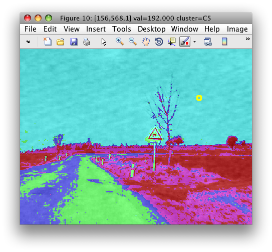
By hovering over the image, we may see that clusters C1 and C3 correspond
mostly to the road, clusters C2 and C4 to grass and the cluster C5 to sky.
Assigning meaningful names to the clusters is the interpretation step. We
may rename the cluster labels directly in the sdimage figure with the
'rename class' command in the right-click menu or use the sdrelab
function to quickly assign descriptive names:
>> b=sdrelab(a,{[1 3],'road',[2 4],'grass',5,'sky'})
  1: C1     -> road
  2: C2     -> grass
  3: C3     -> road
  4: C4     -> grass
  5: C5     -> sky
412160 by 3 sddata, 3 'cluster' groups: 'road'(89354) 'grass'(105134) 'sky'(217672)
We may now build the road detector on our three-class problem. We will model the road class with a Gaussian model and use the other two classes to fix the detector threshold by minimizing the error:
>> pd=sddetect(b,'road',sdgauss)
  1: road   -> road
  2: grass  -> non-road
  3: sky    -> non-road
sequential pipeline     3x1 'Gaussian model+Decision'
 1  Gaussian model          3x1  one class, 1 component
 2  Decision                1x1  thresholding ROC on road at op 1367
The detector may be applied to a new image:
>> im2=sdimage('roadsign11.bmp','sddata')
412160 by 3 sddata, class: 'unknown'

>> c=im2.*pd
412160 by 3 sddata, 2 classes: 'road'(96068) 'non-road'(316092)
The .* operator is a shorthand for execution of pipeline pd returning
decisions and setting these decisions back in the data set.
>> sdimage(c)
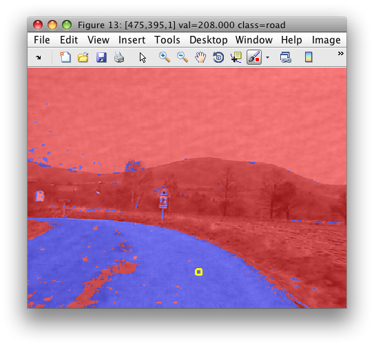
In this example, we used cluster analysis to define meaningful class labels used for training a supervised classifier.
18.2. Clustering with sdcluster command ↩
sdcluster is a high-level command that allows us to perform cluster
analysis on a data set with different clustering algorithms. It accepts a
data set, untrained pipeline of the clustering algorithm and number of
clusters. Optionally, we may provide extra options.
In 3.0.0 release, sdcluster supports only sdkmeans and sdkcentres
clustering algorithms.
Consistently with all other functions in perClass toolbox, sdcluster
executes the clustering algorithm on each class of the current set of
labels:
>> a
'Fruit set' 260 by 2 sddata, 3 classes: 'apple'(100) 'banana'(100) 'stone'(60)

>> b=sdcluster(a,sdkmeans,2)
[class 'apple' 2 clusters] [class 'banana' 2 clusters] [class 'stone' 2 clusters]
'Fruit set' 260 by 2 sddata, 6 'cluster' groups: [61  38  60  48  20  33]
The result is a data set b with cluster labels. Note that sdcluster
does not overwrite the original labels but adds a new 'cluster' property,
setting is as current:
>> b'
'Fruit set' 260 by 2 sddata, 6 'cluster' groups: [61  38  60  48  20  33]
sample props: 'lab'->'cluster' 'class'(L) 'ident'(N) 'cluster'(L)
feature props: 'featlab'->'featname' 'featname'(L)
data props:  'data'(N)
The lab field points to the new 'cluster' labels. The class field
contains the original class labels:
>> b.lab
sdlab with 260 entries, 6 groups:
'C1'(61) 'C2'(38) 'C3'(60) 'C4'(48) 'C5'(20) 'C6'(33)
>> b.class
sdlab with 260 entries, 3 groups: 'apple'(100) 'banana'(100) 'stone'(60)
In this way, we may quickly assess the mapping between the classes and clusters:
>> sdconfmat(b.class,b.lab)

ans =

 True      | Decisions
 Labels    |      C1      C2      C3      C4      C5      C6  | Totals
-----------------------------------------------------------------------
 apple     |     60      32       8       0       0       0   |    100
 banana    |      1       6      43      48       0       2   |    100
 stone     |      0       0       9       0      20      31   |     60
-----------------------------------------------------------------------
 Totals    |     61      38      60      48      20      33   |    260
18.2.1. Clustering all data irrespective of classes ↩
If we wish to cluster the total data set, we may simply set a single class to all samples:
>> c=a
'Fruit set' 260 by 2 sddata, 3 classes: 'apple'(100) 'banana'(100) 'stone'(60)
>> c.lab='unknown'
'Fruit set' 260 by 2 sddata, class: 'unknown'
>> d=sdcluster(c,sdkmeans,2)
[class 'unknown' 2 clusters]
'Fruit set' 260 by 2 sddata, 2 'cluster' groups: 'C1'(102) 'C2'(158)
However, sdcluster provides a faster way with the 'all' option which
executes clustering on all data:
>> a
'Fruit set' 260 by 2 sddata, 3 classes: 'apple'(100) 'banana'(100) 'stone'(60)
>> d2=sdcluster(a,sdkmeans,2,'all')
[class 'Unknown' 2 clusters]
'Fruit set' 260 by 2 sddata, 2 'cluster' groups: 'C1'(150) 'C2'(110)
Original labels are still available:
>> d2.class
sdlab with 260 entries, 3 groups: 'apple'(100) 'banana'(100) 'stone'(60)
18.2.2. How to cluster already clustered data set? ↩
Say we would like to cluster a data set d2 from the previous example
again, now with a different number of clusters:
>> d3=sdcluster(d2,sdkmeans,3)
{??? Error using ==> sdcluster at 59
property 'cluster' is already present in the data set. Choose a different
property for storing clustering result using sdcluster 'lab' option.
}
sdcluster will throw an error because the 'cluster' property is already
present in d2. perClass will never remove a set of labels you created in
the data set. We may either remove the 'cluster' property manually or
simply specify a new name for the property holding clustering result with
'lab' option. Here we store new clustering result in 'newcluster':
>> d3=sdcluster(d2,sdkmeans,3,'lab','newcluster')
[class 'C1' 3 clusters] [class 'C2' 3 clusters]
'Fruit set' 260 by 2 sddata, 6 'newcluster' groups: [42  45  63  39  37  34]
The data set d3 still contains the 'cluster' and 'class' label sets:
>> d3'
'Fruit set' 260 by 2 sddata, 6 'newcluster' groups: [42  45  63  39  37  34]
sample props: 'lab'->'newcluster' 'class'(L) 'ident'(N) 'cluster'(L) 'newcluster'(L)
feature props: 'featlab'->'featname' 'featname'(L)
data props:  'data'(N)
Because sdcluster always adds clustering outcome as new labels, we may
easily compare two clustering results:
>> sdconfmat(d3.cluster,d3.newcluster)

ans =

 True      | Decisions
 Labels    |      C1      C2      C3      C4      C5      C6  | Totals
-----------------------------------------------------------------------
 C1        |     42      45      60       2       0       1   |    150
 C2        |      0       0       3      37      37      33   |    110
-----------------------------------------------------------------------
 Totals    |     42      45      63      39      37      34   |    260
Note that 'C1' and 'C2' names in the rows refer to different clusters than the 'C1' and 'C2' in the columns. Next section shows how to avoid such confusion.
18.2.3. Changing default cluster names ↩
By default, sdcluster uses 'C' as a prefix for cluster names. We may
change it using the 'prefix' option:
>> d4=sdcluster(d2,sdkmeans,3,'lab','newcluster','prefix','D')
[class 'C1' 3 clusters] [class 'C2' 3 clusters]
'Fruit set' 260 by 2 sddata, 6 'newcluster' groups: [57  47  42  34  39  41]
>> sdconfmat(d3.cluster,d4.newcluster)

ans =

 True      | Decisions
 Labels    |      D1      D2      D3      D4      D5      D6  | Totals
-----------------------------------------------------------------------
 C1        |     56      46      42       0       6       0   |    150
 C2        |      1       1       0      34      33      41   |    110
-----------------------------------------------------------------------
 Totals    |     57      47      42      34      39      41   |    260
We may now easily distinguish the clusters in 'cluster' and in 'newcluster' properties.
18.2.4. Removing cluster labels ↩
If you wish to manually remove the 'cluster' property in d2 set from the
example above, note that sdcluster set it as current labels. Therefore,
we first need to set a different property (label set) as current and only
then remove the 'cluster' property:
>> dd=setlab(d2,'class')
'Fruit set' 260 by 2 sddata, 3 classes: 'apple'(100) 'banana'(100) 'stone'(60)
>> dd=rmprop(dd,'cluster')
'Fruit set' 260 by 2 sddata, 3 classes: 'apple'(100) 'banana'(100) 'stone'(60)
The set dd may be now clustered with sdcluster default setting which
will add 'cluster' property.
18.3. Clustering algorithms ↩
This section describes low-level clustering routines available in
perClass. These routines may be used directly, without sdcluster. They
provide a trained model (pipeline) which still needs to be applied to data
to get clustering decisions.
18.3.1. k-means algorithm ↩
The k-means clustering algorithm minimizes within-cluster variability. It
requires the parameter k denoting the number of desired clusters.
Starting from a set of k randomly selected examples as cluster
prototypes, it iteratively defines partitioning of the data set and shifts
these prototypes to means of the new partitions. Note, that some of the
initial k prototypes may disappear in the optimization
process. Therefore, the resulting number of clusters may be lower.
perClass provides high-speed sdkmeans implementation which is scalable to
very large data sets. By default, sdkmeans works as a classifier. If we
train it on a data set, it describes each class by a set of k prototypes
and return 1-NN classifier.
>> a
'Fruit set' 260 by 2 sddata, 3 classes: 'apple'(100) 'banana'(100) 'stone'(60)
>> p=sdkmeans(a,10)
[class 'apple' 3 clusters pruned,  7 clusters]
[class 'banana' 5 clusters pruned,  5 clusters]
[class 'stone' 3 clusters pruned,  7 clusters]
1-NN (k-means prototypes) pipeline 2x3  3 classes, 19 prototypes
Note that it provides three outputs, each for one of the classes in a.
To use sdkmeans for clustering, we need to add the 'cluster' option:
>> p=sdkmeans(a,10,'cluster')
[class 'apple' 10 clusters] [class 'banana' 10 clusters] [class 'stone' 10 clusters]
1-NN (k-means prototypes) pipeline 2x30  30 classes, 30 prototypes
As a result, the pipeline returned has 30 outputs, each returning a distance to one of the 30 prototypes trained. Note that clustering is performed per class - use 'all' option to cluster all data irrespective of classes:
>> p=sdkmeans(a,10,'cluster','all')
[class 'Unknown' 10 clusters]
1-NN (k-means prototypes) pipeline 2x10  10 classes, 10 prototypes
18.3.1.1. Obtaining cluster labels with sdkmeans ↩
To get cluster labels, we need to make p returning decisions with
sddecide and apply the resulting pipeline to the original data:
>> pd=sddecide(p)
sequential pipeline     2x1 '1-NN (k-means prototypes)+Decision'
 1  1-NN (k-means prototypes)    2x10 10 classes, 10 prototypes
 2  Decision               10x1  weighting, 10 classes, 1 ops at op 1

>> dec=a*pd
sdlab with 260 entries, 10 groups

>> dec.list
sdlist (10 entries)
 ind name
   1 C 1
   2 C 2
   3 C 3
   4 C 4
   5 C 5
   6 C 6
   7 C 7
   8 C 8
   9 C 9
  10 C10
In order to get a data set with decisions as new labels dec in one step, use the .* operator:
>> b=a.*pd
'Fruit set' 260 by 2 sddata, 10 classes: [25  37  29  28   9  35  17  27  23  30]
This is roughly analogous to the use of sdcluster:
>> c=sdcluster(a,sdkmeans,10,'all')
[class 'Unknown' 10 clusters]
'Fruit set' 260 by 2 sddata, 10 'cluster' groups: [22  23  34  24  26  20  38  20  25  28]
The only difference of the later approach is that sdcluster included new
'cluster' labels while the data set b got the decisions set into the
current label set referenced via b.lab.
18.3.1.2. Accessing prototypes derived by sdkmeans ↩
The set of prototypes, derived by sdkmeans is stored in the pipeline p:
>> p
1-NN (k-means prototypes) pipeline 2x10  10 classes, 10 prototypes
>> p{1}

ans =

proto: [10x2x10 sddata]

>> proto=p{1}.proto
10 by 2 sddata, 10 classes: [1  1  1  1  1  1  1  1  1  1]

>> proto'
10 by 2 sddata, 10 classes: [1  1  1  1  1  1  1  1  1  1]
sample props: 'lab'->'class' 'class'(L)
feature props: 'featlab'->'featname' 'featname'(L)
data props:  'data'(N)
Because k-means algorithm derives (extracts) new prototypes by averaging original observations, prototypes do not contain any oroginal properties set in the clustered data set. Use k-centers algorithm if you wish to preserve prototype sample properties.
18.3.2. k-centers algorithm ↩
k-centres algorithm selects k prototypes from the original data set by in such a way that the maximum distance within each cluster is minimized. The main difference with respect to the k-means algorithm is that k-centres prototypes are observations existing in the original data, while k-means exctracted new "virtual" prototypes by averaging. Use k-centres if you wish to find typical observations and use further their original properties.
In this example, we set a unique sample id to each sample:
>> a
'Fruit set' 260 by 2 sddata, 3 classes: 'apple'(100) 'banana'(100) 'stone'(60)
>> a.id=1:length(a)
'Fruit set' 260 by 2 sddata, 3 classes: 'apple'(100) 'banana'(100) 'stone'(60)

>> a(127).id

ans =

   127
Now, we cluster the data set with sdkcentres asking for 10 clusters:
>> p=sdkcentres(a,10,'cluster','all')
[class 'unknown' 10 comp]
1-NN (k-centers prototypes) pipeline 2x10  10 classes, 10 prototypes
The derived prototypes contain the id property:
>> p{1}.proto'
'Fruit set' 10 by 2 sddata, 10 'cluster' groups: [1  1  1  1  1  1  1  1  1  1]
sample props: 'lab'->'cluster' 'class'(L) 'ident'(N) 'id'(N) 'cluster'(L)
feature props: 'featlab'->'featname' 'featname'(L)
data props:  'data'(N)
So we may easily identify what samples were selected:
>> p{1}.proto.id

ans =

     8
   235
   246
   185
    66
   207
    62
    71
   174
   117
18.3.3. Gaussian mixture model ↩
Gaussian mixture model available through sdmixture function may be used
for data clustering. It has one substantial advantage with respect to
k-means and k-centres algorithms: sdmixture may automatically select the
number of clusters in the data.
By default, sdmixture operates per class and returns per-class output:
>> p=sdmixture(a)
[class 'apple' initialization: 4 clusters  EM:.............................. 4 comp]
[class 'banana' initialization: 4 clusters  EM:.............................. 4 comp]
[class 'stone' initialization: 1 cluster  EM:.............................. 1 comp]
Mixture of Gaussians pipeline 2x3  3 classes, 9 components
We received three outputs for the three classes in a.
sdmixture with 'cluster' option will return one outputfor each of the
mixture components (clusters) found. The operation is sill on the per-class
basis:
>> p=sdmixture(a,'cluster')
[class 'apple' initialization: 4 clusters  EM:.............................. 4 comp]
[class 'banana' initialization: 4 clusters  EM:.............................. 4 comp]
[class 'stone' initialization: 1 cluster  EM:.............................. 1 comp]
Mixture of Gaussians pipeline 2x9  9 classes, 9 components
If we wish to cluster the whole data set, we may set a single class:
>> a
'Fruit set' 260 by 2 sddata, 3 classes: 'apple'(100) 'banana'(100) 'stone'(60)
>> a.lab='unknown'
'Fruit set' 260 by 2 sddata, class: 'unknown'

>> p=sdmixture(a,'cluster')
[class 'unknown' initialization: 3 clusters  EM:.............................. 3 comp]
Mixture of Gaussians pipeline 2x3  3 classes, 3 components

>> p.lab
sdlab with 3 entries: 'Cluster 1','Cluster 2','Cluster 3'
Assigning data to clusters:
>> pd=sddecide(p)
sequential pipeline     2x1 'Mixture of Gaussians+Decision'
 1  Mixture of Gaussians    2x3  3 classes, 3 components
 2  Decision                3x1  weighting, 3 classes

>> b=a.*pd
'Fruit set' 260 by 2 sddata, 3 classes: 'Cluster 1'(72) 'Cluster 2'(80) 'Cluster 3'(108)
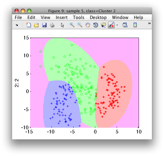
We may visualize the clustering results in the feature space:
>> sdscatter(b,pd)
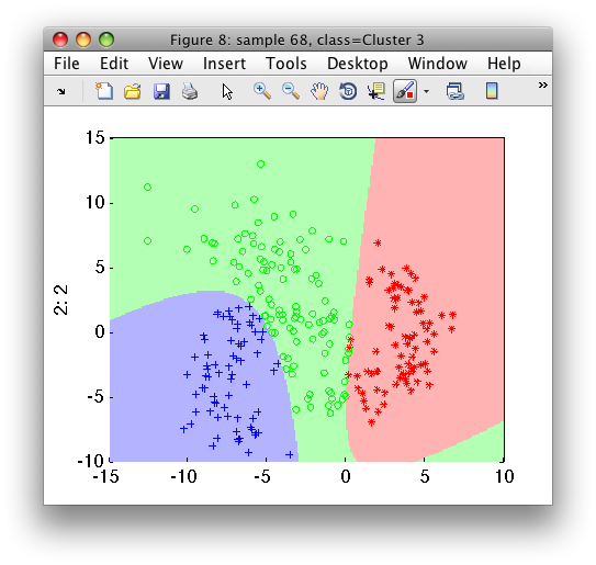
Using pd, any 2D feature vector will be assigned into one of the three
clusters. Sometimes, we may wish to distinguish the feature space domain
observed when performing the clustering from far away outliers or
previously unseen clusters. We may do this by adding reject option to the
pd pipeline:
>> pr=~sdreject`(pd,b)
Weight-based operating point,3 classes,[0.33,0.33,...]
sequential pipeline     2x1 'Mixture of Gaussians+Decision'
 1  Mixture of Gaussians    2x3  3 classes, 3 components (sdp_normal)
 2  Decision                3x1  weight+reject, 4 decisions, ROC 1 ops at op 1 (sdp_decide)

>> sdscatter(b,pr)

>> pr.list
sdlist (4 entries)
 ind name
   1 Cluster 1
   2 Cluster 2
   3 Cluster 3
   4 reject
You may find more detailed discussion on this technique in this blog entry