- 17.1. Classifier combining introduction
- 17.2. Soft-output combining
- 17.2.1. Stacking multiple classifiers
- 17.2.1.1. Creating stack pipelines by concatenation
- 17.2.1.2. Creating stack pipelines from cell arrays
- 17.2.1.3. Accessing base classifiers from the stack
- 17.2.2. Fixed combiners
- 17.2.2.1. Comparable soft output types
- 17.2.2.2. Changing fixed combination rule
- 17.2.3. Trained combiners
- 17.3. Crisp combining of classifier decisions
- 17.3.1. Stacks of classifiers returning decisions
- 17.3.2. Crisp combining with 'all agree' rule
- 17.3.3. Crisp combining with 'at least' rule
- 17.4. Hierarchical classifiers and cascades
This chapter describes combining multiple classifiers.
17.1. Classifier combining introduction ↩
Classifier combining leverages multiple classifiers to improve performance. Combining is known under many other names such as classifier fusion, multiple classifier systems, mixtures of experts etc.
The concept of classifier fusion is quite general. In fact, several perClass classifiers can be considered as compositions of elementary learners. This includes mixtures of Gaussians, decision trees, random forests or neural networks.
In this chapter, we describe different approaches based on fusion of any of the basic models into one system. Two major strategies are discussed:
In the first approach, soft outputs of the base models such as posterior probabilities or distances are combined. In the second, we fuse the crisp decisions.
17.2. Soft-output combining ↩
perClass supports two major approaches to soft-output classifier combining, namely fixed and trained combiners. Fixed combiners are rules chosen on the basis of our assumptions on the problem. For example, if we know that classifiers trained on different data representations are independent, we might choose product rule.
The second type of classifier combiner is trained. Instead of assuming any fusion strategy, we learn it from examples. Trained combiners simply use per-class outputs of base classifiers as new features.
17.2.1. Stacking multiple classifiers ↩
In order to build any combiner, we need to train the base classifiers, and stack them into a single pipeline. Lets consider this example on fruit data:
>> load fruit
260 by 2 sddata, 3 classes: 'apple'(100) 'banana'(100) 'stone'(60)
>> p1=sdquadratic(a)
sequential pipeline       2x1 'Quadratic discriminant'
 1 Gaussian model         2x3  full cov.mat.
 2 Normalization          3x3
 3 Decision               3x1  weighting, 3 classes
>> p2=sdparzen(a)
.....sequential pipeline  2x1 'Parzen model+Decision'
 1 Parzen model           2x3  260 prototypes, h=0.8
 2 Decision               3x1  weighting, 3 classes
The soft outputs of out classifiers are accessible by removing the decision
step. This may be done using an unary - operator:
>> -p1
sequential pipeline       2x3 'Gaussian model+Normalization'
 1 Gaussian model          2x3  full cov.mat.
 2 Normalization           3x3

>> -p2
Parzen model pipeline     2x3  260 prototypes, h=0.8
17.2.1.1. Creating stack pipelines by concatenation ↩
To combine soft outputs, we need to stack multiple classifiers together. This may be achieved using horizontal concatenation operator:
>> ps=[-p1 -p2]
stack pipeline            2x6  2 classifiers in 2D space
Applying our stacking pipeline to the 2D data, we obtain 6D data set:
>> b=a*ps
'Fruit set' 260 by 6 sddata, 3 classes: 'apple'(100) 'banana'(100) 'stone'(60)
The new features correspond to per-class soft outputs of the base classifiers. Because our training set contains three classes, we have apple, banana and stone output from each base classifier:
>> +ps.lab

ans =

apple
banana
stone
apple
banana
stone
17.2.1.2. Creating stack pipelines from cell arrays ↩
Classifier stacks may be also created from a cell array of pipeline using
sdstack command.
>> ps=sdstack({-p1 -p2})
stack pipeline            2x6  2 classifiers in 2D space
17.2.1.3. Accessing base classifiers from the stack ↩
Details on the stacked pipeline can be obtained with the ' transpose operator:
>> ps'
stacked pipeline        2x6 'stack'
 inlab:'1','2'
 1 Gaussian model+Normalization      2x3
   output: posterior
  lab:'apple','banana','stone'
 2 Parzen model                      2x3
   output: probability density
  lab:'apple','banana','stone'
Any pipeline may be extracted from the stack by its index:
>> ps(1)
sequential pipeline       2x3 'Gaussian model+Normalization'
 1 Gaussian model          2x3  full cov.mat.
 2 Normalization           3x3
17.2.2. Fixed combiners ↩
Fixed combiner is a rule applied to soft-outputs of the base classifiers. For example, we may wish to average-out errors of based classifiers. Therefore, we adopt a mean combination rule. It will create new soft output set with averages of each per-class output over all classifiers.
In perClas, fixed combiners are implemented through the sdcombine
function. It takes a stacked pipeline as input and by default uses the mean
combiner:
>> pc=sdcombine([-p1 -p2])
sequential pipeline       2x1 'stack+Fixed combiner+Decision'
 1 stack                  2x6  2 classifiers in 2D space
 2 Fixed combiner         6x3  mean rule
 3 Decision               3x1  weighting, 3 classes
17.2.2.1. Comparable soft output types ↩
It is important to note that all base classifiers must yield comparable soft outputs. Otherwise, the assumptions the combiner is based on do not hold. In our example above, the first base classifier returns posteriors while the second probability densities. These soft-outputs are not comparable.
Here we display soft outputs of our stack pipeline ps on first 10 samples
in data set a:
>> +a(1:10)*ps

ans =

0.9963    0.0032    0.0005    0.0190    0.0012    0.0001
0.9827    0.0171    0.0001    0.0155    0.0011    0.0000
0.9651    0.0252    0.0097    0.0167    0.0007    0.0003
0.9989    0.0011    0.0000    0.0191    0.0004    0.0000
0.9971    0.0028    0.0000    0.0117    0.0004    0.0000
0.9982    0.0016    0.0002    0.0185    0.0011    0.0000
0.9877    0.0120    0.0004    0.0172    0.0021    0.0001
0.9987    0.0012    0.0001    0.0221    0.0006    0.0000
0.9786    0.0152    0.0062    0.0161    0.0003    0.0003
0.9884    0.0112    0.0004    0.0173    0.0020    0.0001
Note that the first three columns sum to one (posteriors) while the last three do not (densities).
One way to make output of probabilist model comparable is to normalize them
into posteriors with sdnorm. Lets us it on the Parzen pipeline p2:
>> sdnorm(-p2)
sequential pipeline       2x3 'Parzen model+Normalization'
 1 Parzen model            2x3  260 prototypes, h=0.8
 2 Normalization           3x3
We recreate the stacked pipeline:
>> ps2=[-p1 sdnorm(-p2)]
stack pipeline            2x6  2 classifiers in 2D space

>> ps2'
stacked pipeline        2x6 'stack'
 inlab:'1','2'
 1 Gaussian model+Normalization      2x3
   output: posterior
  lab:'apple','banana','stone'
 2 Parzen model+Normalization        2x3
   output: posterior
  lab:'apple','banana','stone'

>> pc=sdcombine(ps2)
sequential pipeline       2x1 'stack+Fixed combiner+Decision'
 1 stack                   2x6  2 classifiers in 2D space
 2 Fixed combiner          6x3  mean rule
 3 Decision                3x1  weighting, 3 classes
17.2.2.2. Changing fixed combination rule ↩
The combination rule may be specified in the sdcombine second parameter:
>> pc=sdcombine(ps2,'prod')
sequential pipeline       2x1 'stack+Fixed combiner+Decision'
 1 stack                   2x6  2 classifiers in 2D space
 2 Fixed combiner          6x3  prod rule
 3 Decision                3x1  weighting, 3 classes
Available fixed fusion rules:
- 'mean' - averaging out errors of base models
- 'prod' - product when assuming independence of the base classifiers (e.g. trained in different feature spaces)
- 'min' - choose least sure model
- 'max' - useful to pick the most sure classifier. Classifiers must be properly trained.
17.2.3. Trained combiners ↩
Trained combiner is a second-order classifier trained on a data set comprised of soft-outputs of base classifiers.
The advantage of trained combiners is that we may use any based classifier models even having incompatible soft outputs. For the second stage classifier, soft-outputs are mere new features.
>> a
'Fruit set' 260 by 2 sddata, 3 classes: 'apple'(100) 'banana'(100) 'stone'(60)

>> p1=sdquadratic(a)
sequential pipeline       2x1 'Quadratic discriminant'
 1 Gaussian model          2x3  full cov.mat.
 2 Normalization           3x3
 3 Decision                3x1  weighting, 3 classes

>> p2=sdparzen(a)
.....sequential pipeline       2x1 'Parzen model+Decision'
 1 Parzen model            2x3  260 prototypes, h=0.8
 2 Decision                3x1  weighting, 3 classes

>> ps=[-p1 -p2]
stack pipeline            2x6  2 classifiers in 2D space
Now we create a training set for the combiner. In this example, we reuse all training data:
>> b=a*ps
'Fruit set' 260 by 6 sddata, 3 classes: 'apple'(100) 'banana'(100) 'stone'(60)
The combiner is trained on the set b. We use simple linear discriminant:
>> pf=sdfisher(b)
sequential pipeline       6x1 'Fisher linear discriminant'
 1 LDA                     6x2
 2 Gaussian model          2x3  single cov.mat.
 3 Normalization           3x3
 4 Decision                3x1  weighting, 3 classes
The final classifier is composed of a stack and the combiner:
>> pfinal=ps*pf
sequential pipeline       2x1 'stack+Fisher linear discriminant'
 1 stack                   2x6  2 classifiers in 2D space
 2 LDA                     6x2
 3 Gaussian model          2x3  single cov.mat.
 4 Normalization           3x3
 5 Decision                3x1  weighting, 3 classes
Testing our combined system on the independent set:
>> ts
'Fruit set' 20000 by 2 sddata, 3 classes: 'apple'(6667) 'banana'(6667) 'stone'(6666)
>> sdtest(ts,pfinal)
ans =
0.0920
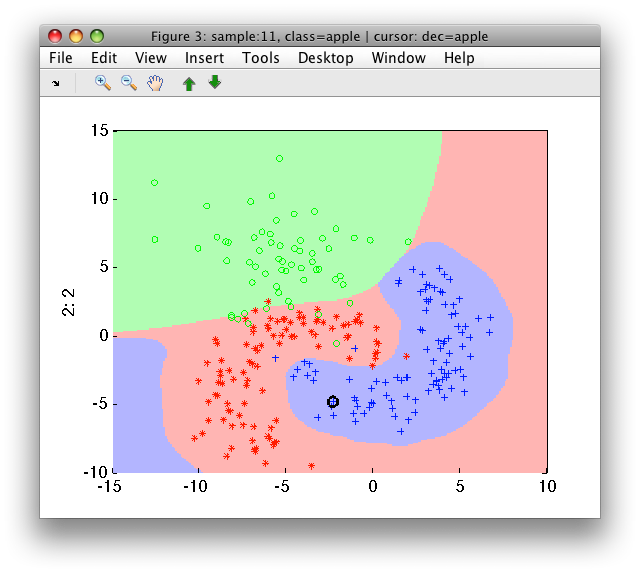
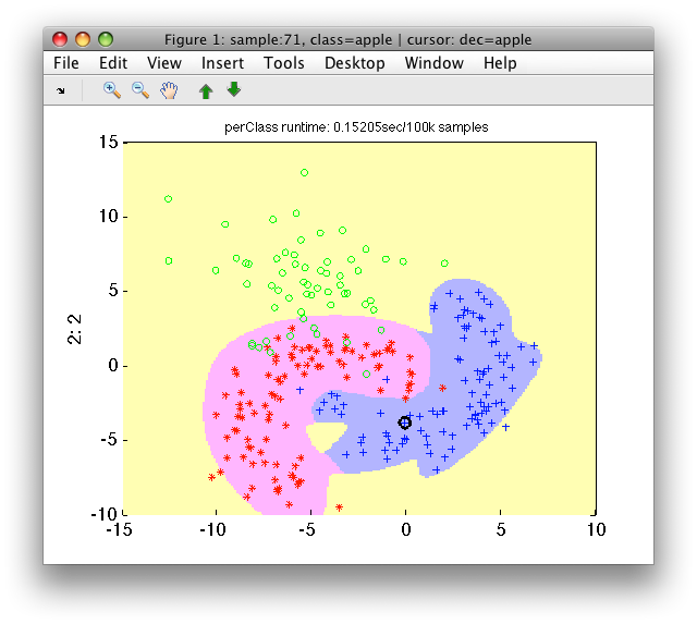
>> sdscatter(a,pfinal)
Note, that reuse of all training data for both stages may result in
over-fitting of the combiner. Multiple strategies are possible such as
validation set approach or stacked generalization (available in perClass
via sdstackgen command).
For details, see e.g. P.Paclik, T.C.W.Landgrebe, D.M.J.Tax, R.P.W.Duin, On deriving the second-stage training set for trainable combiners, in proc. of Multiple Classifier Systems conference MCS 2005
17.3. Crisp combining of classifier decisions ↩
Second major approach of classifier fusion is to combine decisions of base classifiers, not their soft outputs. This has a major advantage in allowing us to optimize each of the base learner for the task at hand with ROC analysis. For example, in a defect detection system, we may tune each base classifier not to loose certain type of defect.
17.3.1. Stacks of classifiers returning decisions ↩
The sdstack function and horizontal concatenation can be used also on
classifiers returning decisions.
Using our example from above, we will fuse the quadratic discriminant with Parzen classifier:
>> p1
sequential pipeline       2x1 'Quadratic discriminant'
 1 Gaussian model          2x3  full cov.mat.
 2 Normalization           3x3
 3 Decision                3x1  weighting, 3 classes
>> p2
sequential pipeline       2x1 'Parzen model+Decision'
 1 Parzen model            2x3  260 prototypes, h=0.8
 2 Decision                3x1  weighting, 3 classes
Note that we provide classifier pipelines directly, without removing the decision steps:
>> pscrisp=[p1 p2]
decision stack pipeline   2x2  2 classifiers in 2D space

>> pscrisp'
stacked pipeline        2x2 'decision stack'
 inlab:'1','2'
 1 Quadratic discriminant            2x1
   output: decision
 list:'apple','banana','stone'
 2 Parzen model+Decision             2x1
   output: decision
 list:'apple','banana','stone'
17.3.2. Crisp combining with 'all agree' rule ↩
The sdcombine command takes a stack of classifiers on its input:
>> pc=sdcombine(pscrisp)
sequential pipeline       2x1 'decision stack+crisp combiner'
 1 decision stack          2x2  2 classifiers in 2D space
 2 crisp combiner          2x1  all agree rule
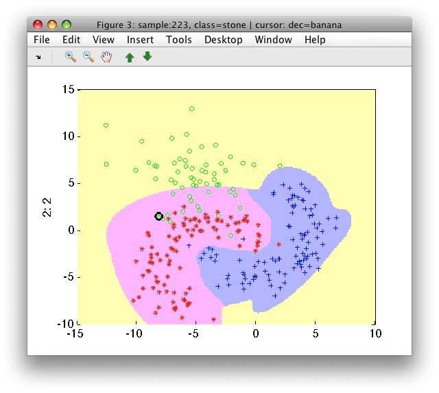
By default, the 'all agree' rule is used. This yields the class output only if all base classifier agree with it. If not, the reject decision is given. We may see the rejected areas in the scatter plot:
>> sdscatter(a,pc)
The reject decision can be adjusted by the 'reject' option:
>> pc=sdcombine(pscrisp,'reject','stone')
sequential pipeline       2x1 'decision stack+crisp combiner'
 1 decision stack          2x2  2 classifiers in 2D space
 2 crisp combiner          2x1  all agree rule
>> sdscatter(a,pc)

17.3.3. Crisp combining with 'at least' rule ↩
An alternative crisp combination rule is 'at least' N agree.
We build a set of 10 decision trees. Recall, that a sdtree performs a
random split inside to get a validation set for pruning. We use this to
introduce some variability in our 10 base classifiers. Without variability
in the models, there is no benefit on fusion.
>> P={}; for i=1:10, P{i}=sdtree(a); end

>> ps=sdstack(P)
decision stack pipeline   2x10  10 classifiers in 2D space
The 'at least' combination rule takes an extra argument specifying how many base classifiers need to agree. We also need to set the target class to avoid tie situations:
>> pc=sdcombine(ps,'at least',8,'target','apple')
sequential pipeline       2x1 'decision stack+crisp combiner'
 1 decision stack          2x10 10 classifiers in 2D space
 2 crisp combiner         10x1  on 'apple' at least 8 of 10

>> sdscatter(a,pc)
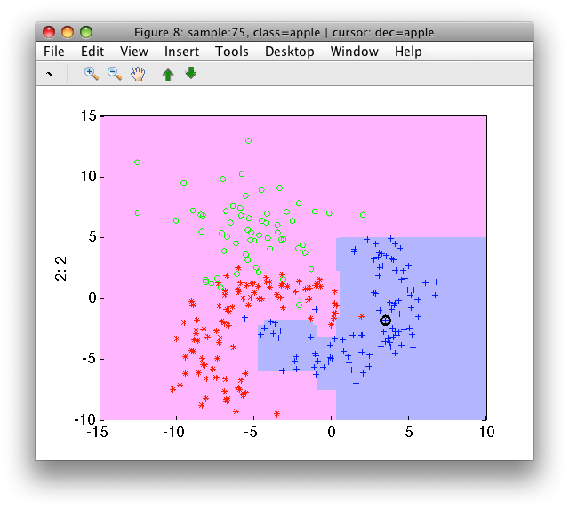
The 'at least' fusion rule is very useful, for example, in purifying high precision decisions in defect detection applications.
17.4. Hierarchical classifiers and cascades ↩
Cascading is a form of classifier combining based on decisions. All
examples, that are labeled with a specific decision are passed to different
classifier. This approach allows us to design multi-stage systems or use
best features for each sub-problem. Classifier hierarchy is built with
sdcascade command.
Let us take an example where we want to build a detector for fruit, followed by classification of specific fruit type.
>> a
'Fruit set' 260 by 2 sddata, 3 classes: 'apple'(100) 'banana'(100) 'stone'(60)
First, we prepare a training set of the fruit detector, joining 'apple' and 'banana' classes into 'fruit':
>> b=sdrelab(a,{'~stone','fruit'})
  1: apple  -> fruit
  2: banana -> fruit
  3: stone  -> stone
'Fruit set' 260 by 2 sddata, 2 classes: 'stone'(60) 'fruit'(200)
Now we train a detector for fruit. We use a mixture model because we know about multi-modality of our 'fruit' class:
>> pd=sddetect(b,'fruit',sdmixture)
[class 'fruit' init:.......... 6 clusters EM:done  6 comp]
  1: stone  -> non-fruit
  2: fruit  -> fruit
sequential pipeline       2x1 'Mixture of Gaussians+Decision'
 1 Mixture of Gaussians    2x1  6 components, full cov.mat.
 2 Decision                1x1  ROC thresholding on fruit (52 points, current 17)
We visualize classifier decisions on the complete set and show also the ROC
plot (stored in the detector pd):
>> sdscatter(a,pd,'roc')

We choose the operating point where we do not loose much of precious fruit
and save it back into the detector pd by pressing 's' key.
>> Setting the operating point 12 in sdppl object pd
sequential pipeline       2x1 'Mixture of Gaussians+Decision'
 1 Mixture of Gaussians    2x1  6 components, full cov.mat.
 2 Decision                1x1  ROC thresholding on fruit (52 points, current 12)
Now we can build a classifier separating 'apple' and 'banana' examples. Lets use Parzen classifier:
>> p2=sdparzen( a(:,:,1:2) )
....sequential pipeline       2x1 'Parzen model+Decision'
 1 Parzen model            2x2  200 prototypes, h=0.6
 2 Decision                2x1  weighting, 2 classes
Our detector returns 'fruit' and 'non-fruit' decisions:
>> pd.list
sdlist (2 entries)
 ind name
   1 fruit
   2 non-fruit
Now we can compose a cascade which first executes the pd detector on all
samples. Samples, labeled 'fruit' will be passed on to the second-stage
classifier p2:
>> pc=sdcascade(pd,'fruit',p2)
Classifier cascade pipeline 2x1  2 stages

>> sdscatter(a,pc)
We can observe that our 'apple'/'banana' classifier is protected from all directions by the first stage detector.
17.4.1. Accessing operating points in a cascade ↩
The cascade is composed of several classifiers returning decisions:
>> pc'
cascaded pipeline       2x1 'Classifier cascade'
 inlab:'Feature 1','Feature 2'
 1 Mixture of Gaussians+Decision     2x1
   dec:'fruit','non-fruit'
 2 Parzen model+Decision             2x1
   applied on: 'fruit'
   dec:'apple','banana'
We may read-out the operating point or point set directly using the ops field:
>> pc(1).ops
Thr-based operating set (52 ops) at op 12
17.4.2. Changing operating points in a cascade ↩
We may set the current operating point directly by providing a desired index from the ROC plot:
>> pc(1).curop=2
Classifier cascade pipeline 2x1  2 stages
This will expand the detector boundary:
>> sdscatter(a,pc)