
Feature extraction, table of contents
- 8.2.1. Introduction
- 8.2.2. Quick example
- 8.2.3. Region feature types
- 8.2.3.1. Raw neighborhood values
- 8.2.3.2. Local mean and standard deviation
- 8.2.3.3. Local histograms
- 8.2.3.4. Features extracted from local histograms
- 8.2.3.5. Co-occurrence matrices
- 8.2.3.6. Gaussian filter and its derivatives
- 8.2.3.7. Sobel filter
- 8.2.3.8. User-defined filter bank
- 8.2.3.9. Leung-Malik multi-orientation/multi-scale filter bank
- 8.2.3.10. Schmid rotationally-invariant filter bank
- 8.2.3.11. Maximum Response filter bank combining multiple orientations
- 8.2.3.12. Maximum Response filter bank combining multiple orientations and scales
- 8.2.3.13. Gray-level morphology features
- 8.2.3.14. User-defined feature extractors
- 8.2.4. Grid definition
- 8.2.5. Visualization of feature images computed on a grid
- 8.2.6. Computing features based on foreground mask
- 8.2.7. Propagating image labels
- 8.2.8. Visualizing regions in original image
8.2.1. Introduction ↩
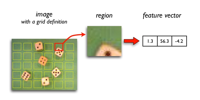
Region feature extractors process square image neighborhoods and represent its central pixel by the resulting feature vector. This is useful to account for local spatial information and structure in images. Typical applications are texture classification and image segmentation (distinguishing edges).
Region features help you to characterize:
- Local texture
- Local intensity distribution (histograms)
- Local gradient, edge strength and orientation
- Response of a convolution filter
- Local appearance
Region feature extraction framework allows you to:
- Compute local image features (several build-in types or custom Matlab extractors)
- Use custom neighborhood sizes and grid definitions
- Work with image masks and irregular image patches
- Propagate existing image labels to extracted data sets
- Visualize label images highlighting image neighborhoods in original images
- Easily pass labels between images extracted at different scales
8.2.2. Quick example ↩
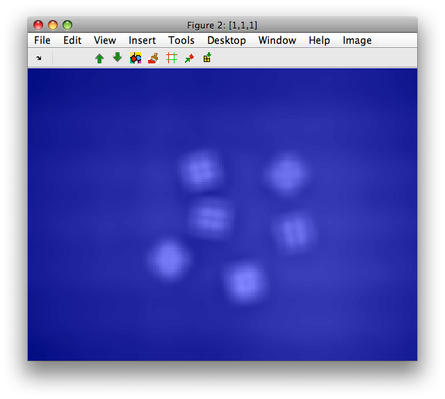
For this example we load a dice image sddata object I:
>> I=sdimage('dice01.jpg','sddata')
101376 by 3 sddata, class: 'unknown'
It becomes a data set with three features corresponding to R,G,B bands respectively.
>> sdimage(I)

ans =

 1
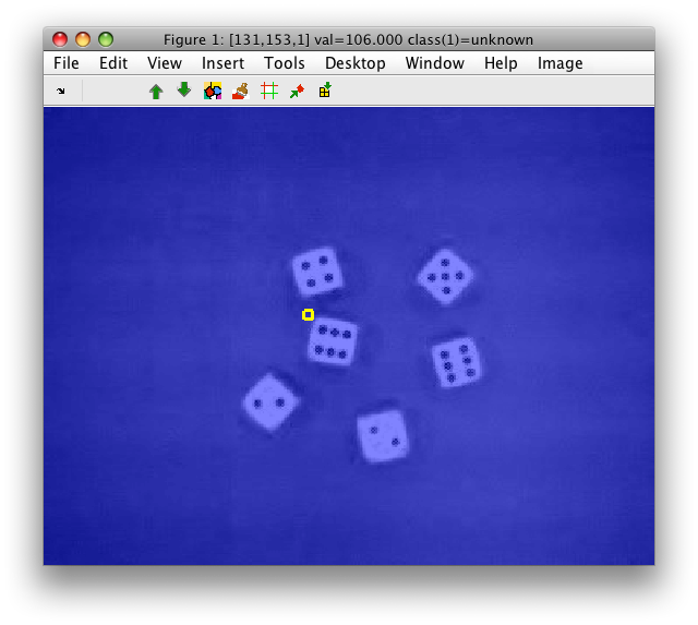
The blue color is the label layer that is uniform, because we have only one "unknown" class by default.
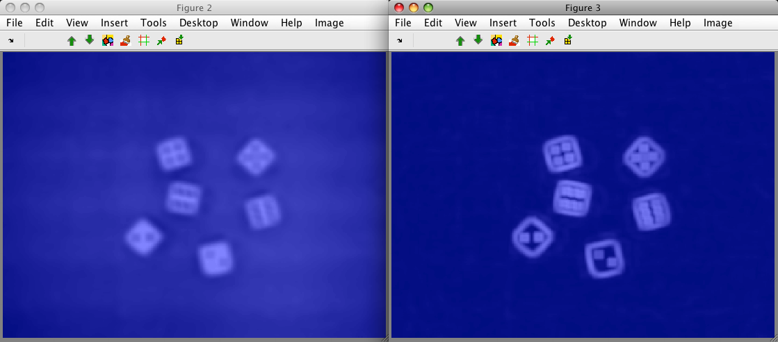
We want to characterize local image structure. The simplest approach is to compute mean and standard deviation in small image neighborhoods with the 'moments' extractor:
 >> A=sdextract( I(:,1), 'region', 'moments')
 96945 by 2 sddata, class: 'unknown'
Note that 'moments' extractor operates on a single image band and we,
therefore, provide it only with the first feature ('R' channel). The
extraction domain is 'region' and the extractor name is 'moments'. By
default, 'moments' features are extracted in 8x8 sliding windows. The
resulting data set A is still an image (see this chapter)
We can visualize it with sdimage. We open two separate figures, one
showing the first feature (local mean), the other showing the second
feature (local standard deviation):
>> sdimage(A)

ans =

 2

>> sdimage(A(:,2))

ans =

 3
Note, that the extracted image contains a thin border without data. This is
because perClass computes region features only if the neighborhood fully
covers image data. For example, the left-upper corner pixel cannot be
represented because the neighborhood "sticks out" from available data.
Therefore, the number of samples in A is slightly smaller that in the
original image I.
Why is local feature extraction useful? Let us try to separate objects and
background by clustering. Move to the Figure 2 that contains data set A
with both bands and select 'Cluster with k-means' from 'Image' menu. Enter
the desired number of clusters, for us 2 and click OK.
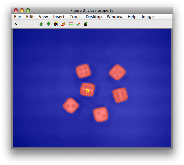
We can observe is that clustering on mean/std features robustly identifies
the dice objects including the dots due to larger spatial context. For
comparison, perform clustering on the original RGB image I or its first
band I(:,1).
8.2.3. Region feature types ↩
8.2.3.1. Raw neighborhood values ↩
- name: 'raw'
- description: Unrolling pixel neighborhood into a feature vector
- use case:
- describe local image structure for small neighborhoods
- applies to: single image channel (input feature)
- required parameter: none
- optional parameters: none
- output dimensionality: input dimensionality squared
- defaults:
- 'block' : 8
- 'step' : 1
Example:
>> im1
262144 by 1 sddata, class: 'unknown'
>> out=sdextract(im1,'region','raw','block',3)
260100 by 9 sddata, class: 'unknown'
8.2.3.2. Local mean and standard deviation ↩
- name: 'moments'
- description: Local mean and standard deviation in the image block
- use case:
- describe intensity variations at local image level (texture characterization)
- average out pixel noise (mean feature)
- highlight edge information (std feature)
- applies to: single image channel (input feature)
- required parameter: none
- optional parameters: none
- output dimensionality: 2
- defaults:
- 'block' : 8
- 'step' : 1
Example: See above.
8.2.3.3. Local histograms ↩
- name: 'hist'
- description: Local histogram in a region
- use case:
- describe intensity variations at local image level (texture characterization)
- applies to: single image channel (input feature)
- required parameter:
- 'range',R : define data range with two-component vector R
[min max]. Values outside the range are discarded.
- 'range',R : define data range with two-component vector R
- optional parameters:
- 'bins',N : number of histogram bins (default: 8)
- output dimensionality: N
- defaults:
- 'block' : 8
- 'step' : 1
The histogram feature extractor requires explicitly specified data
range. It is important that the 'range' is identical in the entire
classification problem i.e. on the training set and in the production or
test set. Therefore, you should not use data-driven definitions such as
'range',[+min(im) +max(im)]! This holds also for other histogram-like
features ('histfeat' and 'cm').
Examples:
>> data=sdextract(I(:,1),'region','hist','range',[0 255])
96945 by 8 sddata, class: 'unknown'

>> data=sdextract(I(:,1),'region','hist','range',[0 255],'bins',16)
96945 by 16 sddata, class: 'unknown'
8.2.3.4. Features extracted from local histograms ↩
- name: 'histfeat'
- description: Statistical features characterizing shape of local histogram in a region
- use case:
- describe intensity variations at local image level (texture characterization)
- applies to: single image channel (input feature)
- required parameter:
- 'range',R : define data range with two-component vector R
[min max]. Values outside the range are discarded.
- 'range',R : define data range with two-component vector R
- optional parameters:
- 'bins',N : number of histogram bins (default: 8)
- output dimensionality: 5
- defaults:
- 'block' : 8
- 'step' : 1
The 'histfeat' extractor computes five statistical features characterizing shape of local histograms. These are: 'mean','2nd moment','skewness','kurtosis', and 'entropy'
>> data=sdextract(I(:,1),'region','histfeat','range',[0 255])
96945 by 5 sddata, class: 'unknown'
>> data.featlab
sdlab with 5 entries, 5 groups:
'Feature 1,mean'(1) 'Feature 1,2nd moment'(1) 'Feature 1,skewness'(1) 'Feature 1,kurtosis'(1) 'Feature 1,entropy'(1)
8.2.3.5. Co-occurrence matrices ↩
Co-occurrence matrix is a two-dimensional histogram estimating probability that a pixel has a specific gray-level while a displaced pixel exhibits another gray-level. Co-occurrence matrix encodes structural information which is useful for derivation of informative data representation in texture classification problems.
- name: 'cm'
- description: Co-occurrence matrix
- use case:
- describe local image structure/texture for texture classification
- applies to: single image channel (input feature)
- required parameter:
- 'range',R : define data range with two-component vector R
[min max]. Values outside the range are discarded.
- 'range',R : define data range with two-component vector R
- optional parameters:
- 'bins',N : number of co-occurrence bins (default: 8). Smaller values are more common as they yield less sparse matrices.
- 'displ',D : pixel displacement in vertical direction (default: 1). Number of pixels at which we record the gray-level relations.
- output dimensionality: N^2
- defaults:
- 'block' : 8
- 'step' : 1
In this example, we compute co-occurrences on R channel, subsampling intensities to 4 bins:
>> data=sdextract(I(:,1),'region','cm','range',[0 255],'bins',4)
96945 by 16 sddata, class: 'unknown'
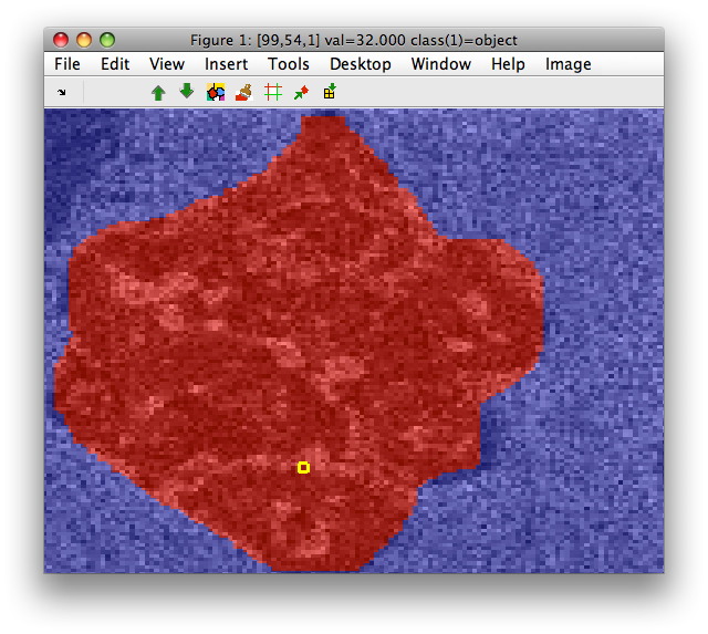
Let is identify pixel row 101, column 162 in our data set. We can use standard Matlab sub2ind function and imsize of our image:
>> ind=sub2ind(getiminfo(data,'imsize'),101,162)

ind =

   46469
Now we get the sample with pixel index ind:
>> data( data.pixel==ind )
1 by 16 sddata, class: 'unknown'
Co-occurrence as feature vector:
>> +data( data.pixel==ind )

ans =

  Columns 1 through 7

     0    0.0089    0.0089    0.0089    0.0089         0         0

  Columns 8 through 14

0.0179    0.0089         0    0.0179    0.0268    0.0089    0.0179

  Columns 15 through 16

0.0268    0.8393
and reshaped into 4x4 matrix:
>> reshape(ans,[4 4])

ans =

     0    0.0089    0.0089    0.0089
0.0089         0         0    0.0179
0.0089         0    0.0179    0.0268
0.0089    0.0179    0.0268    0.8393
8.2.3.6. Gaussian filter and its derivatives ↩
- name: 'gauss'
- description: response of convolving image with Gaussian filter or its derivative
- use case:
- noise removal, focus on larger-scale structure in the image (with larger sigma)
- highlighting edges/local image gradients (with derivatives)
- applies to: single image channel (input feature)
- required parameter: none
- optional parameters:
- 'sigma',S : smoothing parameter of the Gaussian filter (default: 2.0)
- 'der',D : derivative (default: D=0). D may be scalar or vector with two components with different derivative for rows and columns, resp.
- output dimensionality: 1
- defaults:
- 'block' : 8
- 'step' : 1
The 'gauss' feature extractor convolves input image with Gaussian filter or its derivative and returns its response in the central pixel of each image region.
By default, sigma of 2 and block of 8 pixels are used:
% using the dice01.jpg image loaded above
>> data=sdextract(I(:,1),'region','gauss')
block: 8, sigma: 2.0 yields kernel coverage 91.5%
96945 by 1 sddata, class: 'unknown'
Note the message displaying the actual coverage of the convolution kernel on the image region. Gaussian kernel has in general an infinite support. In practice, we only use the convolution values in the neighborhood defined by the 'block' option. Therefore our filter only covers the sliding window partially.
If we use larger sigma, the coverage gets lower which means that our actual filtering result is getting further away from ideal Gaussian shape:
>> data=sdextract(I(:,1),'region','gauss','sigma',3)
block: 8, sigma: 3.0 yields kernel coverage 67.2%
96945 by 1 sddata, class: 'unknown'
In order to increase the coverage, we may increase the 'block' size:
>> data=sdextract(I(:,1),'region','gauss','sigma',3,'block',12)
block: 12, sigma: 3.0 yields kernel coverage 91.3%
94457 by 1 sddata, class: 'unknown'
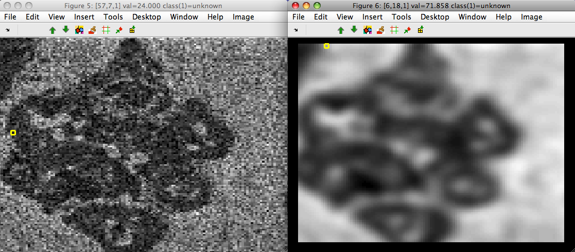
Example on 'detergent1' data set illustrating the noise suppression:
>> load detergent1
>> imdet=sdimage(im1m,'sddata')
16384 by 7 sddata, class: 'unknown'

>> data=sdextract(imdet(:,1),'region','gauss','sigma',3,'block',12)
block: 12, sigma: 3.0 yields kernel coverage 91.3%
13689 by 1 sddata, class: 'unknown'
>> sdimage(imdet)

ans =

 5

>> sdimage(data)

ans =

 6
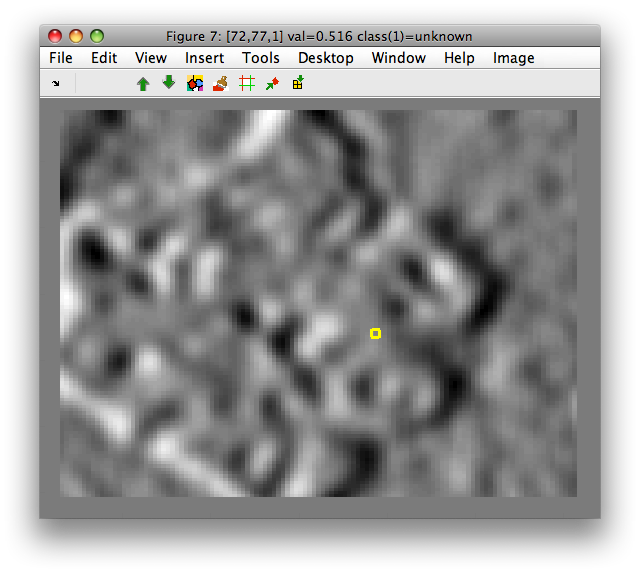
Gaussian derivatives are also supported with 'der' option:
>> data2=sdextract(imdet(:,1),'region','gauss','sigma',3,'block',12,'der',[1 0])
block: 12, sigma: 3.0 yields kernel coverage 91.3%
13689 by 1 sddata, class: 'unknown'
>> sdimage(data2)

ans =

 7
8.2.3.7. Sobel filter ↩
- name:, 'sobel' or 'sobel.x','sobel.y','sobel.mag'
- description: Sobel operator computing local image gradient
- use case:
- identify edges
- applies to: single image channel (input feature)
- required parameter: none
- optional parameters: none
- output dimensionality:
- 'sobel' : 2 features (gradient magnitude, gradient orientation)
- 'sobel.x' : 1 feature (gradient filter response in x direction (rows) )
- 'sobel.y' : 1 feature (gradient filter response in xy direction (columns) )
- 'sobel.mag' : 1 feature1 (gradient magnitude only)
- defaults:
- 'block' : 3 (cannot be changed by 'block', use 'gauss' before for larger scales.)
- 'step' : 1
Sobel filter computes local image gradient in 3x3 image neighborhoods.
>> data=sdextract(imdet,'region','sobel')
15876 by 2 sddata, class: 'unknown'

>> sdimage(imdet)
>> sdimage(im)
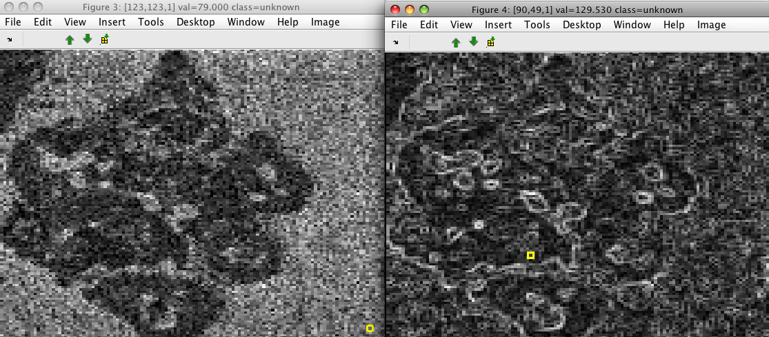
The data set contains two features. The first describes gradient magnitude and the second its orientation:
>> data.featlab
sdlab with 2 entries, 2 groups: 'Feature 1,gradient magnitude'(1) 'Feature 1,gradient orientation'(1)
In order to highlight larger-scale structures, we may want to filter the image first with a Gaussian:
>> data1=sdextract(imdet(:,1),'region','gauss','sigma',3,'block',16)
block: 16, sigma: 3.0 yields kernel coverage 98.5%
12769 by 1 sddata, class: 'unknown'

>> data2=sdextract(data1,'region','sobel')
12321 by 2 sddata, class: 'unknown'

>> sdimage(data2(:,1))
>> sdimage(data2(:,2))
The result of directional Sobel filters may be extracted using the 'sobel.x' and 'sobel.y' options, respectively:
>> x=sdextract(imdet(:,1),'region','sobel.x')
15876 by 1 sddata, class: 'unknown'
8.2.3.8. User-defined filter bank ↩
- name:, 'fbank'
- description: User-defined convolutional filter bank
- use case:
- describe local texture/structure/edges
- applies to: single image channel (input feature)
- required parameter: 'kernel',K to define 3D kernel matrix
- optional parameters: 'join',F
- output dimensionality: size(K,3)
- defaults:
- 'step' : 1
Filter bank is specified with 3D matrix K (block x block x
filter_count). The 'fbank' extractor supports maximum response filtering
with 'join' option. To define it, a vector F should be supplied with one
entry per filter. Each entry in F specifies to which final output (joined
filter) is this filter merged.
8.2.3.9. Leung-Malik multi-orientation/multi-scale filter bank ↩
- name:, 'fbank:LM'
- description: A set of 48 multi-scale/multi-orientation filters
- use case:
- describe local texture
- applies to: single image channel (input feature)
- required parameter: none
- optional parameters: none
- output dimensionality: 48
- defaults:
- 'block' : 49 (cannot be changed)
- 'step' : 1
Example:
>> im1
986049 by 1 sddata, class: 'unknown'
>> out=sdextract(im1,'region','fbank:LM')
893025 by 48 sddata, class: 'unknown'
LM filters:

Reference: http://www.robots.ox.ac.uk/~vgg/research/texclass/filters.html
8.2.3.10. Schmid rotationally-invariant filter bank ↩
- name:, 'fbank:S'
- description: A set of 13 multi-scale rotationally-invariant filters
- use case:
- describe local texture
- applies to: single image channel (input feature)
- required parameter: none
- optional parameters: none
- output dimensionality: 13
- defaults:
- 'block' : 49 (cannot be changed)
- 'step' : 1
Schmid filters:

8.2.3.11. Maximum Response filter bank combining multiple orientations ↩
- name:, 'fbank:MR8'
- description: A set of 8 filters, 6 respond to lines (arbitrarily oriented) at different scales, 2 are rotationally-invariant filters
- use case:
- describe local line structures and texture
- applies to: single image channel (input feature)
- required parameter: none
- optional parameters: none
- output dimensionality: 8
- defaults:
- 'block' : 49 (cannot be changed)
- 'step' : 1
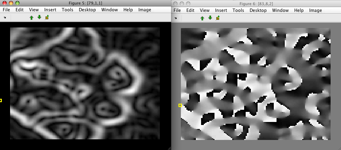
In this example, we extract MR8 filter bank on an image combining multiple Brodatz textures:
 >> im1=sdimage('texmos1.p512.tiff','sddata')
 262144 by 1 sddata, class: 'unknown'

 >> out=sdextract(im1,'region','fbank:MR8')
 215296 by 8 sddata, class: 'unknown'

 >> sdimage(out); sdimage(im1);
The figure shows original image and one output feature i.e. combined output of multiple orientation filters.

8.2.3.12. Maximum Response filter bank combining multiple orientations and scales ↩
- name:, 'fbank:MR4'
- description: A set of 4 filters, 2 respond to lines combining different orientations and scales, 2 are rotationally-invariant filters
- use case:
- describe local line structures and texture
- applies to: single image channel (input feature)
- required parameter: none
- optional parameters: none
- output dimensionality: 4
- defaults:
- 'block' : 49 (cannot be changed)
- 'step' : 1
8.2.3.13. Gray-level morphology features ↩
Gray-level morpology enables straightforward edge detection in single-band images. It uses a square structure element with a size defined by the 'block' option. At the low level, erosion and dilation operations are defined similar to the classical black and white morphology. On top of these, opening and closing operations are specified. The high-level 'edge' extractor uses opening and closing to enhance edge regions.
- name:, 'edge'
- description: Enhancing edge regions
- use case:
- define object boundaries and edge regions
- applies to: single image channel (input feature)
- required parameter: none
- optional parameters: none
- output dimensionality: 1
- defaults:
- 'block' : 8
- 'step' : 1
8.2.3.14. User-defined feature extractors ↩
Apart from built-in feature extractors, sdextract can execute a custom
Matlab function on each image neighborhood. This allows us to quickly
experiment with arbitrary external code for feature computation while
benefiting from the flexible image grid definition and masking.
To use custom feature extractor, we need to create a Matlab function
following a specific syntax. As an example, lets define a function
custom_extract_hist.m that will compute a local image histogram in each
region.
The custom feature extractor is invoked by providing function handle instead of extractor name:
>> data=sdextract(im,'region',@custom_extract_hist)
..........
14641 by 8 sddata, class: 'unknown'
In our example, we want to be able to set the number of histogram bins, and data range for the histograms estimated. These are the extractor parameters.
To provide parameters, we simply pass a cell array with name, value pairs after the function handle:
>> data=sdextract(im,'region',@custom_extract_hist,{'bins',16,'min',0,'max',255})
..........
14641 by 16 sddata, class: 'unknown'
How to implement the custom feature extractor function?
Any feature extraction function needs to do two things:
- Set extraction parameter and return feature names (called once)
- Extract feature vector from a given neighborhood (called many times)
Our function will have, as any custom callback function, two inputs and two outputs:
function [data,par]=custom_extract_hist(data,par)

if isempty(data)

    % 1. parameter setting
    %     - (optional) set any default params or precomputed data used
    %       during block processing
    %     - return feature labels

    % set default number of bins
    if ~isfield(par,'bins')
    par.bins=8;
    end
    % set default minimum and maximum value
    if ~isfield(par,'min')
    par.min=0;
    end
    if ~isfield(par,'max')
    par.max=255;
    end

    % store the histogram bins definition
    par.histbins=par.min:floor((par.max-par.min+1)/par.bins):par.max;

    % return feature labels
    data=sdlab('Hist ',1:par.bins);

else

    % 2. block processing
    %     - process input block matrix data and return feature vector
    % data is a image block (matrix)
    % par is a struct with parameters

    A=data(:);

    data=hist(A,par.edge)./sum(A);

end
The first part is called by sdextract once, before the block-by-block
feature computation, to initialize any parameters our extractor need and
return the feature labels. The data input argument is empty, the par
argument is a structure with some basic fields describing the extraction
process, such as block size and step.
We may add any further fields to par. In our example, we set the bins,
min, and max fields to default values, in not already present.
We also create anything we need for feature extraction process. In our
example, it is useful to define the histogram binning vector histbins
once.
Finally, we return the feature labels.
The second part of the extractor function is called for each image
neighborhood. The data argument is now a neighborhood matrix and par
our parameter structure with all fields we set. Now we perform the
computation and return the feature vector.
Note, that feature extraction process is not limited to single-band
images. If the input image data set, passed to sdextract has multiple
bands, the custom function will receive a 3D matrix for each
neighborhood. In this way, you may implement e.g. color texture features or
process hyperspectral images in one pass.
8.2.4. Grid definition ↩
Region features are computed on a regular grid laid over an image. The grid is defined by two parameters:
- block size
- grid step
Block size is an scalar defining the square sliding window. Default value is 8 (8x8 pixel regions). It may be changed using the 'block' option.
The default step is 1. Large step is useful for representing large images as it yields sparse smaller representation.
>> B=sdextract(I(:,1),'region','moments','block',16)
92001 by 2 sddata, class: 'unknown'

>> C=sdextract(I(:,1),'region','moments','block',16,'step',2)
23153 by 2 sddata, class: 'unknown'
The getiminfo method can be used to access detailed information on grid
definition for any image data set.
>> getiminfo(I)

ans =

imsize: [288 352]

>> getiminfo(C)

ans =

  imsize: [288 352]
    grid: 1
   block: 16
    step: 2
gridsize: [137 169]
Typical use-case for getiminfo is to return directly image size:
>> s=getiminfo(C,'imsize')

s =

   288   352
8.2.5. Visualization of feature images computed on a grid ↩
The sdimage command visualizes any image data set in the context of the
''original image''. Therefore, data extracted on a grid with step higher
than one will be sparse:
>> sdimage(C)

ans =

 1

Note the gaps between data points. We may wish to remove the grid pattern for the sake of visualization purposes. This may be done using 'Shrink to grid' command in Image menu:
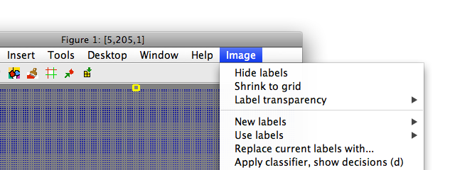
A new figure window opens with out image constrained to grid.
We can achieve the same from the command prompt with the sdimage 'grid'
option:
>> D=sdimage(C,'grid')
23153 by 2 sddata, class: 'unknown'
>> sdimage(D)

ans =

 2

>> getiminfo(D)

ans =

imsize: [137 169]
8.2.6. Computing features based on foreground mask ↩
Often, we only want to process certain part of an image, e.g. object that was already segmented out from the conveyor belt by low-level image processing.
sdextract accepts the 'mask' option that specifies where to compute the
features.
Lets assume we have a object mask as a set of labels in out data set:
Our mask label M:
>> M
sdlab with 16384 entries, 2 groups: 'object'(8207) 'background'(8177)
We may extract features only from the region defined by this mask. The 'mask' option takes, as argument a logical vector or image matrix.
If our mask is represented by label object, we may just compare it to the desired class resulting in a logical vector:
>> out=sdextract(imdet(:,1),'region','moments','mask',M=='object')
6667 by 2 sddata, class: 'unknown'
>> sdimage(out)
Features are computed only for neighborhoods that fully cover available
image data. Therefore, the resulting data set out contains less samples
than the 'object' class in M.
If our mask is a matrix such as objmask:
>> objmask=reshape(-M,getiminfo(imdet,'imsize'));
>> size(objmask)

ans =

   128   128
Numerical representation of our labels contain 1-based indices:
>> unique(objmask(:))

ans =

 1
 2
Because 'object' was first in the M.lab.list (see above), we can define our mask with:
>> out=sdextract(imdet(:,1),'region','moments','mask',objmask==1)
6667 by 2 sddata, class: 'unknown'
8.2.7. Propagating image labels ↩
When applied to sddata data set with image data, sdextract
propagates image labels and all sample properties to the output data.
We may, for example, define labels my hand, painting directly in the sdimage
figure. In this example, we painted background, particle and "interesting
texture" regions. We save the data set in Matlab workspace using Image menu:
>> sdimage(imdet)
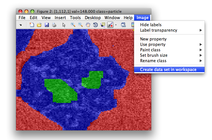
>> Creating data set data2 in the workspace.
16384 by 1 sddata, 3 classes: 'background'(7629) 'particle'(7760) 'interesting texture'(995)
We may now compute the features on data set data2. The class labels get
propagated to the pixels that serve as block centers in feature
computation:
>> a=sdextract(data2(:,1),'region','histfeat','block',4)
15625 by 5 sddata, 3 classes: 'background'(7517) 'particle'(7113) 'interesting texture'(995)

>> sdimage(a)
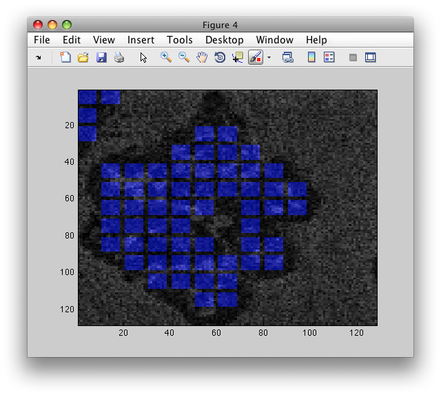
8.2.8. Visualizing regions in original image ↩
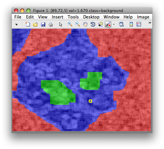
When extracting features from local image neighborhoods, we often want to visualize the exact block position in the original image. For example, this is very useful in order to understand, what parts of the object are misclassified.
The label image shows the image neighborhoods in the context of the original image, used for feature extraction.
Say, we start from the particle image with the segmented background:
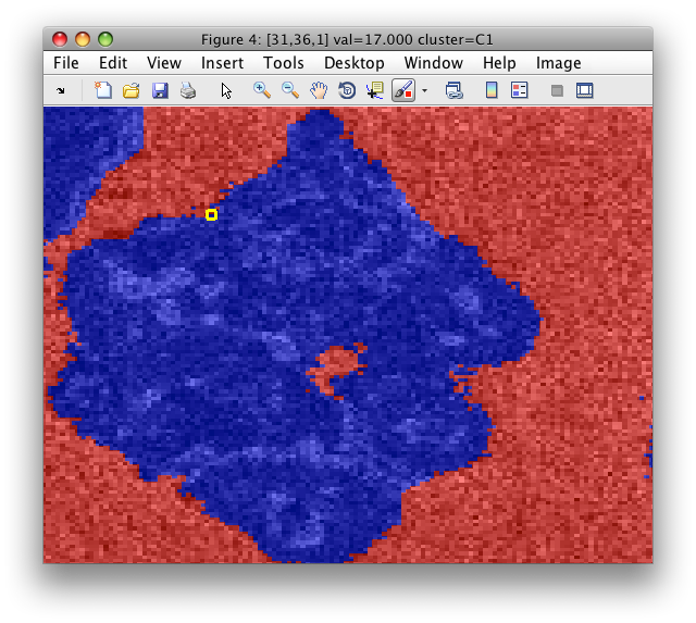
We save the image data set into Matlab workspace as data2:
>> Creating data set data2 in the workspace.
16384 by 7 sddata, 2 'cluster' groups: 'C1'(8263) 'C2'(8121)
We only use the C1 cluster (the particle foreground):
>> sub=data2(:,:,'C1')
8263 by 7 sddata, 'cluster' lab: 'C1'
Now, we compute features on the first band of the particle:
>> b=sdextract(sub(:,1),'region',@custom_extract_hist,'block',8,'step',10)
..........
60 by 8 sddata, 'cluster' lab: 'C1'
To visualize block positions, use sdimage with 'labim' option. It will
extract RGB image of the same size at the original image and impaint blocks
with colors based on the labels b.lab:
>> LI=sdimage(b,'labim');
>> figure; imagesc(LI)
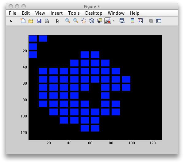
Note the gap inside the particle. As mentioned above, sdextract computes
features only in regions without holes.
We may wish to visualize the label image blended with the original image
with 'blend' option. We provide image matrix with <0,1> values with the
same dimensions as the original image (imsize in getiminfo(b)).
>> LI=sdimage(b,'labim','blend',I./256);
>> figure; imagesc(LI)
To adjust image blending, use 'alpha' parameter:
>> LI=sdimage(b,'labim','blend',I./256,'alpha',0.8);
>> figure; imagesc(LI)
Finally, to use different set of labels than the b.lab, you may provide
the any sdlab object with the same length directly after the
'labim' option. This is useful when visualizing decisions (we assume a
classifier p trained on extracted features):
>> dec=b*p
>> LI=sdimage(b,'labim',dec,'blend',I./256,'alpha',0.8);
>> figure; imagesc(LI)