Keywords: detectors, cascade of classifiers, ROC analysis

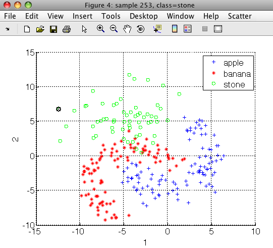
The gendatf function generates an artificial dataset with three classes (apple,banana and stone, representing the outliers). Note that we need labeled outliers (here stones) to optimize the detector with ROC analysis.

>> load fruit; a 
Fruit set, 260 by 2 dataset with 3 classes: [100  100   60]

In order to build the fruit detector, we construct a two-class problem with fruit and stone classes using sdrelab:

>> b=sdrelab(a,{'~stone','fruit'})
  1: apple  -> fruit 
  2: banana -> fruit 
  3: stone  -> stone
'Fruit set' 260 by 2 sddata, 2 classes: 'stone'(60) 'fruit'(200) 
>> [pd,r1]=sddetector(b,'fruit',sdgauss)
  1: stone  -> non-fruit
  2: fruit  -> fruit    
sequential pipeline     2x1 'Gaussian model+Decision'
 1  Gaussian model          2x1  one class, 1 component (sdp_normal)
 2  Decision                1x1  thresholding ROC on fruit at op 13 (sdp_decide)
ROC (52 thr-based op.points, 3 measures), curop: 13
est: 1:err(fruit)=0.05, 2:err(non-fruit)=0.17, 3:mean-error=0.11

Because we specify a target class which is present in the sddata b, sddetector uses the remaining class(es) as non-targets and adopts the ROC analysis to fix the operating point. By default, the target model is trained on 80% of the data, and the ROC is estimated on the remaining 20%. The ROC is returned in the second output of sddetector. We will now train the apple/banana discriminant. In order to estimate the ROC, we will split the available data in two parts manually:

>> c=a(:,:,{'apple','banana'});
'Fruit set' 200 by 2 sddata, 2 classes: 'apple'(100) 'banana'(100) 
>> [tr,ts]=randsubset(c,0.8); 
>> r2=sdroc(ts*sdquadratic(tr))   %  estimate ROC on the subset of c
ROC (41 w-based op.points, 3 measures), curop: 1
est: 1:err(apple)=0.00, 2:err(banana)=0.20, 3:mean-error=0.10
>> p=sdquadratic(c);    %  re-train the classifier on all available data
>> pd2=p*r2
 1  Gauss full cov.         2x2  2 classes, 2 components (sdp_normal)
 2  Output normalization    2x2  (sdp_norm)
 3  Decision                2x1  weighting, 2 classes, ROC 41 ops at op 1 (sdp_decide)

The cascade is constructed by providing the trained detector, the pass-through decision and the discriminant. The detector already includes all operating points estimated by the ROC analysis. For the dicriminant, we fix the operating point explicitly from the ROC r2.

>> pc=sdp_cascade(pd,'fruit',pd2) 
2-stage cascade pipeline 2x1   (sdp_cascade)

We will now open the scatter plot showing cascade decisions. When provided with ROC objects, the sdscatter will open two interactive ROC plots and link them to the scatter. In this way, we can analyze the cascade behaviour at different operating points.

>> sdscatter(a,pc,'roc', {r1 r2}) 

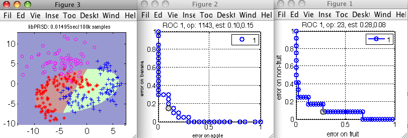
To fix a specific operating point in the cascade, you can press s key in the ROC plot and enter the name of the variable (here pd for the detector, and r2 for the discriminant). We must then re-create the pipeline:

Setting the operating point 11 in sdppl object pd
 1  Gauss full cov.         2x2  2 classes, 2 components (sdp_normal)
 2  Output normalization    2x2  (sdp_norm)
 3  Decision                2x1  weighting, 2 classes, ROC 41 ops at op 11 (sdp_decide)

Setting the operating point 1143 in sdroc object r2
ROC (2001 w-based op.points, 3 measures), curop: 1143
est: 1:err(apple)=0.10, 2:err(banana)=0.15, 3:mean-error=0.12
>> pc=sdp_cascade(pd,'fruit',p*r2) 
>> sdconfmat(a.lab,a*pc) 

ans =

 True      | Decisions
 Labels    | apple  banana non-fr  | Totals
--------------------------------------------
 apple     |    81     15      4   |   100
 banana    |    16     81      3   |   100
 stone     |     0     13     47   |    60
--------------------------------------------
 Totals    |    97    109     54   |   260