
Keywords: image data, PCA, classifier, outliers, classifier execution
23.1. Introduction ↩
This example shows how to approach a typical image classification problem. Suppose, we wish to classify handwritten digit from pre-segmented images.
23.2. Data set ↩
We consider a handwritten digits data set containing 2000 images of ten digit classes scaled to 16x16 matrix. Because pixels are directly used as features, the data set contains 256 dimensions.
>> load digits
>> a
'Digits' 2000 by 256 sddata, 10 classes: [200  200  200  200  200  200  200  200  200  200]
Each image is labeled into one of the digit classes.
>> a.lab
sdlab with 2000 entries, 10 groups
>> a.lab'
 ind name size percentage
   1 0     200 (10.0%)
   2 1     200 (10.0%)
   3 2     200 (10.0%)
   4 3     200 (10.0%)
   5 4     200 (10.0%)
   6 5     200 (10.0%)
   7 6     200 (10.0%)
   8 7     200 (10.0%)
   9 8     200 (10.0%)
  10 9     200 (10.0%)
We will split the data set into training and test subsets. In this way, we will be able to test classifier performance on images unused when training the models.
>> [tr,ts]=randsubset(a,0.5)
'Digits' 1000 by 256 sddata, 10 classes: [100  100  100  100  100  100  100  100  100  100]
'Digits' 1000 by 256 sddata, 10 classes: [100  100  100  100  100  100  100  100  100  100]
23.3. Visualizing the data set ↩
Because the features represent directly the pixels the resulting feature space is very sparse. We will use the principal component analysis (PCA) to extract a lower-dimensional subspace where the data may be easier visualized.
We will use sdpca command and request it to find projection to 40D
subspace of the original 256D space.
>> p=sdpca(tr,40)
PCA pipeline            256x40  73% of variance (sdp_affine)
The result of sdpca is a pipeline object p. We may see, that projecting
into the 40D subspace, we retain 73% of the total variance in the data.
We may now project the training data set into this 40D subspace by
multiplying the original set tr by the pipeline p:
>> tr2=tr*p
'Digits' 1000 by 40 sddata, 10 classes: [100  100  100  100  100  100  100  100  100  100]
In order to understand our data set, we use the sdscatter command:
>> sdscatter(tr2)
It shows all training samples for the two first principal components. Using the cursor keys, we may change features on the horizontal and vertical axes. By pressing 'l' (legend), we show the class names.
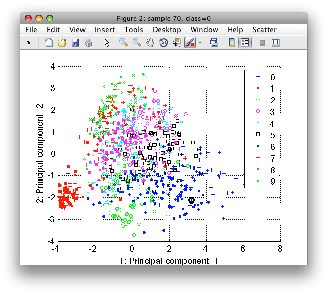
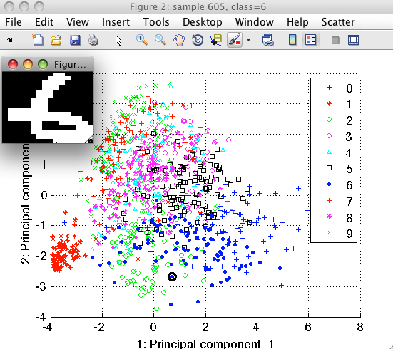
By moving the mouse over the figure, we focus the closes sample with the
black round cursor. We may see both sample index and its class in the
Figure title. The sdscatter also allows us to visualize the original
images under the sample cursor. Use Scatter menu/Show sample inspector
command and fill in the name of the data set containing original images
(tr in our example). A small image window will open showing the data
sample under cursor.
Sample inspector allows us to better understand our data. Lets, for example, consider the digit "1". We position mouse over the examples of class "1" and using the right-mouse-click open the context menu. By selecting "Show only this class" we let the scatter to hide other classes.
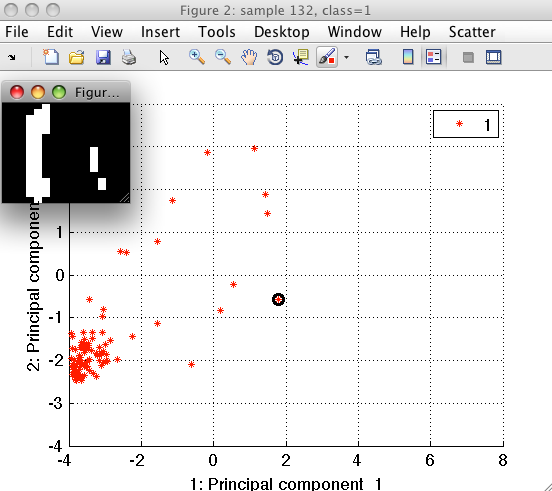
We can see that the outliers of class "1" are either shifted with respect to the center of the bounding box or contain segmentation artifacts.
If we wish to remove such cases from training, we may label the outliers using "Paint class/Create new class" command, hide them and save the clean data set back in Matlab workspace. You may see the example of such outlier removal in this video.
23.4. Building a digit classifier ↩
We will now build a digit classifier. It is a good practice to start by
designing simple models as they often exhibit high robustness and may serve
as a reference baseline when designing more sophisticated classifiers. One
such classical classifier is Fisher linear discriminant (sdfisher).
It derives a linear subspace maximizing separation between the classes and trains a linear Gaussian classifier in it.
>> p2=sdfisher(tr2)
sequential pipeline     40x10 'Fisher linear discriminant'
 1  LDA                    40x9  (sdp_affine)
 2  Gauss eq.cov.           9x10 10 classes, 10 components (sdp_normal)
 3  Output normalization   10x10 (sdp_norm)
We may now put together the complete classifier, composed of PCA projection and the Fisher discriminant:
>> pd=sddecide(p*p2)
sequential pipeline     256x1 'PCA+LDA+Gauss eq.cov.+Output normalization+Decision'
 1  PCA                   256x40 73%% of variance (sdp_affine)
 2  LDA                    40x9  (sdp_affine)
 3  Gauss eq.cov.           9x10 10 classes, 10 components (sdp_normal)
 4  Output normalization   10x10 (sdp_norm)
 5  Decision               10x1  weighting, 10 classes, 1 ops at op 1 (sdp_decide)
Note, that we explicitly state that our classifier pd should return
decisions using the sddecide command. If we omitted sddecide, the
pipeline would return soft output (confidences), not crisp decisions.
Our classifier is now ready to be executed on any data with 256 features. Here, we apply it to the test set and obtain decisions
>> dec=ts*pd
sdlab with 1000 entries, 10 groups
We will use sdtest function to estimate mean class error:
>> sdtest(ts.lab,dec)

ans =

    0.1510
The Fisher classifier yields 15% error on the test set.
We may quickly test a different classifier type, for example, the k-nearest neighbor.
>> p2=sdknn(tr2,5)
5-NN classifier (dist) pipeline 40x10   (sdp_knn)

>> pd2=p*p2*sddecide
sequential pipeline     256x1 'PCA+5-NN classifier (dist)+Decision'
 1  PCA                   256x40 73%% of variance (sdp_affine)
 2  5-NN classifier (dist)   40x10 (sdp_knn)
 3  Decision               10x1  weighting, 10 classes, 1 ops at op 1 (sdp_decide)

>> sdtest(ts,pd2)

ans =

0.1240
Our 5-NN yields better performance than the Fisher classifier above. Note
that we may pass to the sdtest the test set and the trained pipeline
instead of the labels and decisions.
23.5. Understanding the classifier results ↩
Training a classifier is but one step in overall system design. It is important, that we understand in more detail how our classifier works and, especially, where it fails.
To get a more detailed view, we may display a confusion matrix:
>> sdconfmat(ts.lab,ts*pd2)

ans =

 True      | Decisions
 Labels    |       0       1       2       3       4       5       6       7       8       9  | Totals
-------------------------------------------------------------------------------------------------------
 0         |     94       2       3       0       0       0       1       0       0       0   |    100
 1         |      0      95       1       0       2       0       2       0       0       0   |    100
 2         |      2       1      92       0       0       0       0       2       2       1   |    100
 3         |      0       1       2      88       0       3       0       2       3       1   |    100
 4         |      0       8       2       0      71       0       0       2       1      16   |    100
 5         |      1       0       1       1       0      92       2       0       0       3   |    100
 6         |      0       4       1       1       0       0      94       0       0       0   |    100
 7         |      1       1       0       0       1       0       0      87       0      10   |    100
 8         |      0       8       1       9       2       1       0       4      70       5   |    100
 9         |      0       1       1       0       2       0       0       3       0      93   |    100
-------------------------------------------------------------------------------------------------------
 Totals    |     98     121     104      99      78      96      99     100      76     129   |   1000
We may notice, that our k-NN rule misclassified higher number of 4's into 9's. Can we see, what examples go wrong?
We will use the sdconfmatind command to find indices of digit '4' labeled as '9':
>> ind=sdconfmatind(ts.lab,ts*pd2,'4','9');
Now, we will create a new set of labels called 'err' copying the class labels and mark the misclassified examples so we may easily inspect them.
>> ts.err=ts.lab
'Digits' 1000 by 256 sddata, 10 classes: [100  100  100  100  100  100  100  100  100  100]

>> ts.err(ind)='4-err'
'Digits' 1000 by 256 sddata, 10 classes: [100  100  100  100  100  100  100  100  100  100]
The ts.err labels now contain 11 groups:
>> ts.err
sdlab with 1000 entries, 11 groups

>> ts.err'
 ind name     size percentage
   1 0         100 (10.0%)
   2 1         100 (10.0%)
   3 2         100 (10.0%)
   4 3         100 (10.0%)
   5 4          84 ( 8.4%)
   6 5         100 (10.0%)
   7 6         100 (10.0%)
   8 7         100 (10.0%)
   9 8         100 (10.0%)
  10 9         100 (10.0%)
  11 4-err      16 ( 1.6%)
Let us now open the scatter plot and inspect the errors more closely:
>> sdscatter(ts*p)
Go to 'Scatter' menu and choose 'Use property'. You will see that two sets of labels are present, namely 'lab' and 'err'. Select 'err' and switch on the legend by pressing 'l' key.
Now we need to select only the relevant subset of classes, i.e. '4','9', and '4-err'. You may do it by choosing them in the 'Scatter'/'Sample filter' menu. Faster way to specify a subset of classes is to press the '/' key and entering the substrings we are interested in. In our case, we may enter '4|9' meaning "all classes that contain 4 OR 9 in their names".
We may now open the sample inspector on the ts data set and investigate
in detail what shapes of 4's get mixed with 9's.
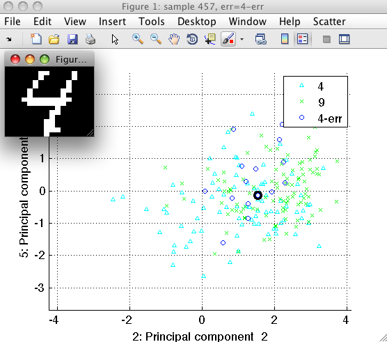
Often, such an analysis of errors helps us to develop more powerful features addressing the specific problem.
23.6. Using the classifier in custom application ↩
When we are happy with our digit classifier, we wish to run it in our custom application. To do that, we use perClass Runtime which allows us to call any classifier we train from arbitrary application.
In our example, we implemented a simple GUI application in RealBasic which allows us to interactively draw digits in 16x16 image and run a classifier. When implementing the GUI, we do not need to decide for the classifier type. We only fix the dimensionality our classifier expects to the 256 input features representing the pixels.
On the side of perClass Toolbox, running in Matlab, we will export our
classifier into a pipeline file using sdexport command:
>> sdexport(pd2,'digit_classifier.ppl')
Exporting pipeline..ok
This pipeline requires perClass runtime version 3.0 (18-jun-2011) or higher.
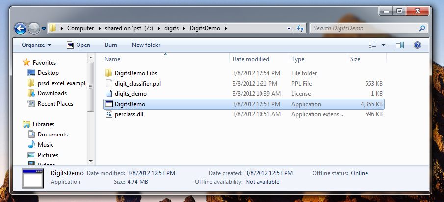
Outside Matlab, we can see the directory with all GUI application files.
The DigitsDemo and DigitsDemo Libs contains the application code,
perclass.dll is the perClass Runtime library and digits_classifier.ppl
is the exported classifier pipeline.
We will now execute the DigitsDemo.exe:
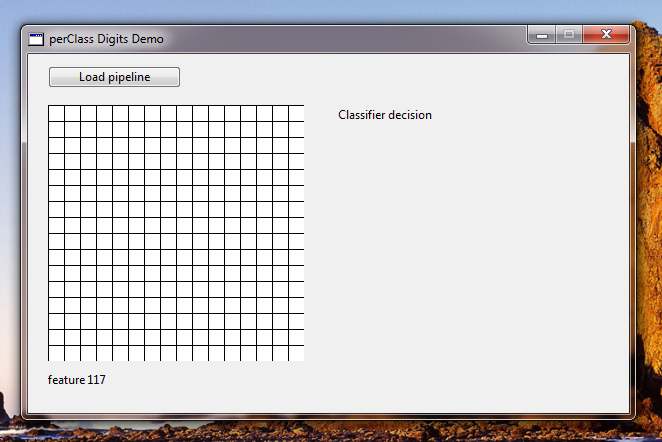
We will load a pipeline and may start drawing digits on the 16x16 grid.
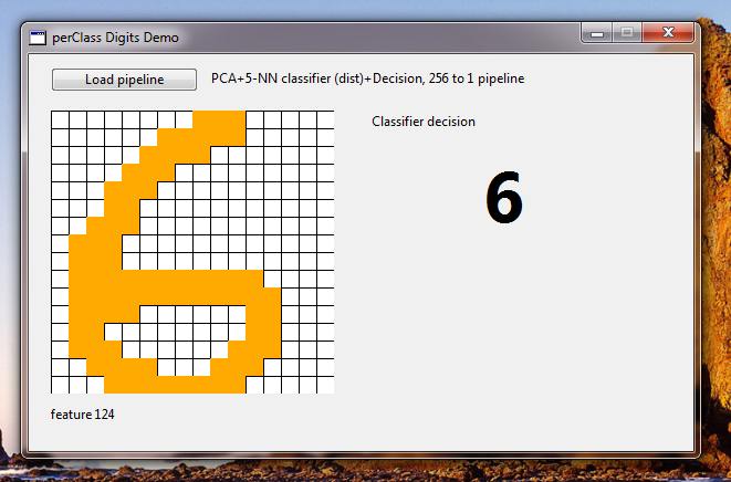
You may now return back to Matlab, update your classifier, re-export it and immediately experience the changes in the live demo.
This concludes our example.