
Keywords: confusion matrices, meta-data
26.1. Confusion matrices ↩
Confusion matrix is an indispensable tool to understand the structure of classifier errors.
In this article, we show several practical tools in perClass getting the most of confusion matrices:
- Constructing a confusion matrix
- Fixing the order of rows and columns
- Extracting samples in a specific matrix field
- Visualize data set structure with confusion matrices
- Cleaning and replacing confusion matrix content
26.1.1. Constructing a confusion matrix ↩
Lets consider, for example, a medical data set:
>> a
'medical D/ND' 5762 by 10 sddata, 2 classes: 'no-disease'(4267) 'disease'(1495)
The data set contains measurements from 16 patients:
>> a.patient
sdlab with 5762 entries, 16 groups
We will use the first 8 to train a classifier and the remaining ones to estimate its performance:
>> [tr,ts]=subset(a,'patient',1:8)
'medical D/ND' 2920 by 10 sddata, 2 classes: 'no-disease'(2032) 'disease'(888)
'medical D/ND' 2842 by 10 sddata, 2 classes: 'no-disease'(2235) 'disease'(607)

>> sdscatter(tr)
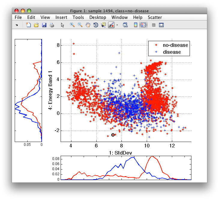
We can see that the classes are quite complex and, therefore, decide to use non-parametric Parzen classifier that does not impose any class shape assumptions. We train Parzen classifier on the training subset:
>> p=sdparzen(tr)
Parzen pipeline         10x2  2 classes, 2920 prototypes (sdp_parzen)
And add a decision output with sddecide function:
>> pd=sddecide(p)
sequential pipeline     10x1 'Parzen+Decision'
 1  Parzen                 10x2  2 classes, 2920 prototypes (sdp_parzen)
 2  Decision                2x1  weighting, 2 classes, 1 ops at op 1 (sdp_decide)
If executed on new data, the pipeline pd returns decisions:
>> dec=ts*pd
sdlab with 2842 entries, 2 groups: 'no-disease'(1527) 'disease'(1315)
We construct the confusion matrix by providing true labels on the test set and the decisions of our classifier on the same samples:
>> sdconfmat(ts.lab,dec)

ans =

 True        | Decisions
 Labels      |  no-dis  diseas  | Totals
-----------------------------------------
 no-disease  |   1479     756   |   2235
 disease     |     48     559   |    607
-----------------------------------------
 Totals      |   1527    1315   |   2842
The confusion matrix shows how the decisions in columns fit the true classes in rows. For example, we can see that 48 disease samples were misclassified as no-disease.
26.1.2. Fixing the order of rows and columns ↩
Notice, that the classes and decisions are given in the order present in our test set and classifier, respectively. This may not be ideal. For example, in medical problems we consider 'disease' class as 'positive'. Therefore, we would like that it is first in the list so that the upper left corner of confusion matrix refers to true positives (correctly found disease).
The sdconfmat command allows us to specify the order of classes and
decisions to make sure all our confusion matrices are comparable.
We may simply provide a cell array in desired order through 'classes' and 'decisions' options:
>> sdconfmat(ts.lab,dec,'classes',{'disease','no-disease'},'decisions',{'disease','no-disease'})

ans =

 True        | Decisions
 Labels      |  diseas  no-dis  | Totals
-----------------------------------------
 disease     |    559      48   |    607
 no-disease  |    756    1479   |   2235
-----------------------------------------
 Totals      |   1315    1527   |   2842
If we assign output of sdconfmat into a variable, we obtain a numerical matrix:
>> CM=sdconfmat(ts.lab,dec,'classes',{'disease','no-disease'},'decisions',{'disease','no-disease'})

CM =

     559          48
     756        1479
With 'classes' and 'decisions' order fixed, we are sure that CM(1,1) refers to true positives and CM(2,1) to false positives.
This feature becomes even more important in everyday life where some of your test sets do not contain all the classes. For example, the last patient in our test set does not have any known diseased tissue (lucky man!). Default confusion matrix would have a different shape:
>> sub=subset(ts,'patient',8)
'medical D/ND' 400 by 10 sddata, class: 'no-disease'

>> sdconfmat(sub.lab,sub*pd)

ans =

 True        | Decisions
 Labels      |  no-dis  diseas  | Totals
-----------------------------------------
 no-disease  |    135     265   |    400
-----------------------------------------
 Totals      |    135     265   |    400
With the 'classes' and 'decisions' options, we make sure the output is square and correctly ordered:
>> sdconfmat(sub.lab,sub*pd,'classes',{'disease','no-disease'},'decisions',{'disease','no-disease'})

ans =

 True        | Decisions
 Labels      |  diseas  no-dis  | Totals
-----------------------------------------
 disease     |      0       0   |      0
 no-disease  |    265     135   |    400
-----------------------------------------
 Totals      |    265     135   |    400
26.1.3. Extracting samples in a specific matrix field ↩
How do we find out what samples are false positives in the previous
example? We may use the sdconfmatind command providing the true labels
and decisions and asking for a specific class/decision combination:
>> ind=sdconfmatind(sub.lab,sub*pd,'no-disease','disease');
>> length(ind)

ans =

   265
The samples may be accessed easily by:
>> sub(ind)
'medical D/ND' 265 by 10 sddata, class: 'no-disease'
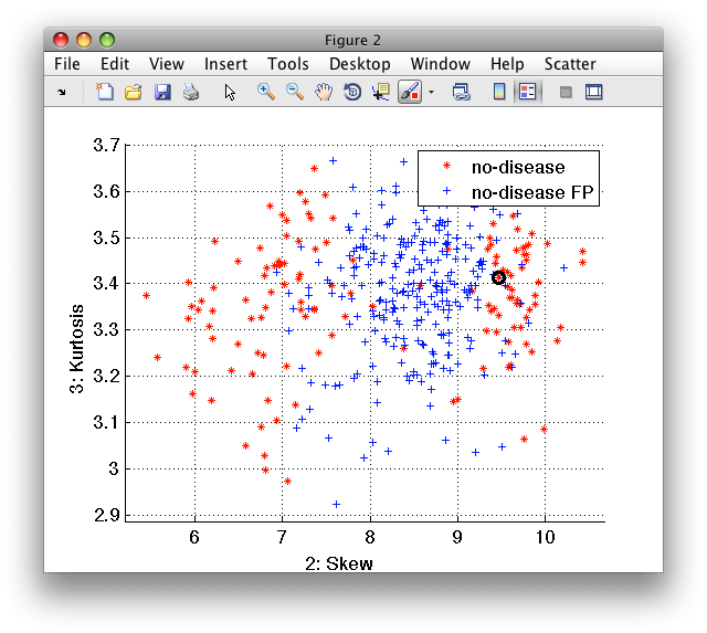
We may, for example, change their label to easily visualize them in scatter plot:
>> sub(ind).lab='no-disease FP'
'medical D/ND' 400 by 10 sddata, 2 classes: 'no-disease'(135) 'no-disease FP'(265)
>> sdscatter(sub)
26.1.4. Visualize data set structure with confusion matrices ↩
We usually think about a confusion matrix as a tool describing true labels and classifier decisions. However, we may also use it with great benefit on any two sets of labels representing the same objects.
For example, we may quickly check the mapping of patients to classes:
>> sdconfmat(ts.patient, ts.lab)

ans =

 True      | Decisions
 Labels    |  no-dis  diseas  | Totals
---------------------------------------
 Irene     |    285      20   |    305
 Monica    |    160      61   |    221
 Nick      |    297      19   |    316
 Olaf      |    336      64   |    400
 Paul      |     86     314   |    400
 Rob       |    362      38   |    400
 Steffany  |    309      91   |    400
 Tom       |    400       0   |    400
---------------------------------------
 Totals    |   2235     607   |   2842
Note the last heathy patient "Tom" we saw in the previous sections.
26.1.5. Clean and replace confusion matrix content ↩
For the last example, I kept one really special option of sdconfmat. We
may easily alter the displayed confusion matrix output with string
replacement rules.
Imagine we work with a multi-class problems such as digit recognition:
>> load digits
>> a
'Digits' 2000 by 256 sddata, 10 classes: [200  200  200  200  200  200  200  200  200  200]
>> a.lab'
 ind name size percentage
   1 0     200 (10.0%)
   2 1     200 (10.0%)
   3 2     200 (10.0%)
   4 3     200 (10.0%)
   5 4     200 (10.0%)
   6 5     200 (10.0%)
   7 6     200 (10.0%)
   8 7     200 (10.0%)
   9 8     200 (10.0%)
  10 9     200 (10.0%)
We train a classifier and get a confusion matrix on the whole set:
>> p=sdpca([],10)*sdparzen*sddecide
untrained pipeline 3 steps: sdpca+sdparzen+sdp_decide

>> pd=a*p
.sequential pipeline     256x1 'PCA+Parzen+Decision'
 1  PCA                   256x10 44%% of variance (sdp_affine)
 2  Parzen                 10x10 10 classes, 2000 prototypes (sdp_parzen)
 3  Decision               10x1  weighting, 10 classes, 1 ops at op 1 (sdp_decide)

>> sdconfmat(a.lab,a*pd)

ans =

 True      | Decisions
 Labels    |       0       1       2       3       4       5       6       7       8       9  | Totals
-------------------------------------------------------------------------------------------------------
 0         |    179       1       1       2       3       7       7       0       0       0   |    200
 1         |      0     178       0       0       6       0       8       4       1       3   |    200
 2         |      1       2     179       5       2       1       1       1       7       1   |    200
 3         |      0       1       1     181       1       3       0       3       6       4   |    200
 4         |      0      13       2       0     153       1       3       1       4      23   |    200
 5         |      5       0       6      14       8     152       2       4       5       4   |    200
 6         |      1      12       3       0       1       1     181       0       1       0   |    200
 7         |      1       1       0       0       1       0       0     173       2      22   |    200
 8         |      0       9       1      11       3       9       0       1     160       6   |    200
 9         |      0       0       1       0      11       1       1       6       5     175   |    200
-------------------------------------------------------------------------------------------------------
 Totals    |    187     217     194     213     189     175     203     193     191     238   |   2000
The matrix is not too readable, especially, if we normalize it by the rows so that the entries represent error rates or performances:
>> sdconfmat(a.lab,a*pd,'norm')

ans =

 True      | Decisions
 Labels    |       0       1       2       3       4       5       6       7       8       9  | Totals
-------------------------------------------------------------------------------------------------------
 0         |  0.895   0.005   0.005   0.010   0.015   0.035   0.035   0.000   0.000   0.000   | 1.00
 1         |  0.000   0.890   0.000   0.000   0.030   0.000   0.040   0.020   0.005   0.015   | 1.00
 2         |  0.005   0.010   0.895   0.025   0.010   0.005   0.005   0.005   0.035   0.005   | 1.00
 3         |  0.000   0.005   0.005   0.905   0.005   0.015   0.000   0.015   0.030   0.020   | 1.00
 4         |  0.000   0.065   0.010   0.000   0.765   0.005   0.015   0.005   0.020   0.115   | 1.00
 5         |  0.025   0.000   0.030   0.070   0.040   0.760   0.010   0.020   0.025   0.020   | 1.00
 6         |  0.005   0.060   0.015   0.000   0.005   0.005   0.905   0.000   0.005   0.000   | 1.00
 7         |  0.005   0.005   0.000   0.000   0.005   0.000   0.000   0.865   0.010   0.110   | 1.00
 8         |  0.000   0.045   0.005   0.055   0.015   0.045   0.000   0.005   0.800   0.030   | 1.00
 9         |  0.000   0.000   0.005   0.000   0.055   0.005   0.005   0.030   0.025   0.875   | 1.00
-------------------------------------------------------------------------------------------------------
Many of the entries are small numbers that only obscure the bigger picture.
With the 'replace' option of sdconfmat, we may specify how some strings
in the final matrix will get replaced. For example, we may turn each 0.000
string into a simple dash:
>> sdconfmat(a.lab,a*pd,'norm','replace',{'0.000','  -  '})

ans =

 True      | Decisions
 Labels    |       0       1       2       3       4       5       6       7       8       9  | Totals
-------------------------------------------------------------------------------------------------------
 0         |  0.895   0.005   0.005   0.010   0.015   0.035   0.035     -       -       -     | 1.00
 1         |    -     0.890     -       -     0.030     -     0.040   0.020   0.005   0.015   | 1.00
 2         |  0.005   0.010   0.895   0.025   0.010   0.005   0.005   0.005   0.035   0.005   | 1.00
 3         |    -     0.005   0.005   0.905   0.005   0.015     -     0.015   0.030   0.020   | 1.00
 4         |    -     0.065   0.010     -     0.765   0.005   0.015   0.005   0.020   0.115   | 1.00
 5         |  0.025     -     0.030   0.070   0.040   0.760   0.010   0.020   0.025   0.020   | 1.00
 6         |  0.005   0.060   0.015     -     0.005   0.005   0.905     -     0.005     -     | 1.00
 7         |  0.005   0.005     -       -     0.005     -       -     0.865   0.010   0.110   | 1.00
 8         |    -     0.045   0.005   0.055   0.015   0.045     -     0.005   0.800   0.030   | 1.00
 9         |    -       -     0.005     -     0.055   0.005   0.005   0.030   0.025   0.875   | 1.00
-------------------------------------------------------------------------------------------------------
That helps a bit. However, most of entries are still small numbers that are not really important to gain overall understanding.
The nice thing about sdconfmat replace is that it may contain any regular
expression. For example, '0.00\d' means: '0.00' followed by one
digit. This helps us to remove entries smaller than 1%:
>> sdconfmat(a.lab,a*pd,'norm','replace',{'0.00\d','  -  '})

ans =

 True      | Decisions
 Labels    |       0       1       2       3       4       5       6       7       8       9  | Totals
-------------------------------------------------------------------------------------------------------
 0         |  0.895     -       -     0.010   0.015   0.035   0.035     -       -       -     | 1.00
 1         |    -     0.890     -       -     0.030     -     0.040   0.020     -     0.015   | 1.00
 2         |    -     0.010   0.895   0.025   0.010     -       -       -     0.035     -     | 1.00
 3         |    -       -       -     0.905     -     0.015     -     0.015   0.030   0.020   | 1.00
 4         |    -     0.065   0.010     -     0.765     -     0.015     -     0.020   0.115   | 1.00
 5         |  0.025     -     0.030   0.070   0.040   0.760   0.010   0.020   0.025   0.020   | 1.00
 6         |    -     0.060   0.015     -       -       -     0.905     -       -       -     | 1.00
 7         |    -       -       -       -       -       -       -     0.865   0.010   0.110   | 1.00
 8         |    -     0.045     -     0.055   0.015   0.045     -       -     0.800   0.030   | 1.00
 9         |    -       -       -       -     0.055     -       -     0.030   0.025   0.875   | 1.00
-------------------------------------------------------------------------------------------------------
If we want to get rid of entries smaller than 5%, we may specify '0.0[01234]\d' pattern saying '0.0' followed by any digit from the list [01234] and later by any arbitrary digit:
>> sdconfmat(a.lab,a*pd,'norm','replace',{'0.0[01234]\d','  -  '})

ans =

 True      | Decisions
 Labels    |       0       1       2       3       4       5       6       7       8       9  | Totals
-------------------------------------------------------------------------------------------------------
 0         |  0.895     -       -       -       -       -       -       -       -       -     | 1.00
 1         |    -     0.890     -       -       -       -       -       -       -       -     | 1.00
 2         |    -       -     0.895     -       -       -       -       -       -       -     | 1.00
 3         |    -       -       -     0.905     -       -       -       -       -       -     | 1.00
 4         |    -     0.065     -       -     0.765     -       -       -       -     0.115   | 1.00
 5         |    -       -       -     0.070     -     0.760     -       -       -       -     | 1.00
 6         |    -     0.060     -       -       -       -     0.905     -       -       -     | 1.00
 7         |    -       -       -       -       -       -       -     0.865     -     0.110   | 1.00
 8         |    -       -       -     0.055     -       -       -       -     0.800     -     | 1.00
 9         |    -       -       -       -     0.055     -       -       -       -     0.875   | 1.00
-------------------------------------------------------------------------------------------------------
This last solution lets us to get a quick insight into overlap patterns in our problem.