
Problem: How to choose a good classifier for multi-modal problem?
Solution: Start simple, test models of growing complexity.
In this example, we walk through a process of finding a good classifier for strongly multi-modal problem. We quickly inspect several families of classifiers and evaluate their accuracy, training and execution speed.
29.1. Introduction ↩
Often, we are faced with clearly multi-modal classification problems where some of the classes are defined in terms of multiple underlying processes. For example, in medical diagnostic problems, we observe that both healthy and diseased tissued come in number of varieties leading to complex shapes of classes in the feature space. In this example, we take a strongly multi-modal problem and discuss how to find a good classifier for it.
We use MNist digit data set that was extensively studied by many machine learning researchers. This data set contains 10 classes of handwritten digit images scaled to 28x28 pixel raster.
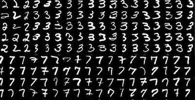
Example of digit images found in the MNist data set:
The data set in sddata format contains 70000 digit images labeled in 10 classes:
>> a
70000 by 784 sddata, 10 classes: [6903  7877  6990  7141  6824  6313  6876  7293  6825  6958]

>> a.lab'
 ind name size percentage
   1 0    6903 ( 9.9%)
   2 1    7877 (11.3%)
   3 2    6990 (10.0%)
   4 3    7141 (10.2%)
   5 4    6824 ( 9.7%)
   6 5    6313 ( 9.0%)
   7 6    6876 ( 9.8%)
   8 7    7293 (10.4%)
   9 8    6825 ( 9.8%)
  10 9    6958 ( 9.9%)
Apart of class labels, the data set contains also the trts_flag providing
the training/test split to 60000/10000 samples used in most of the papers
and the digit id linking each sample to a matrix row in the original
mfeat_all.mat file.
>> a'
70000 by 784 sddata, 10 classes: [6903  7877  6990  7141  6824  6313  6876  7293  6825  6958]
sample props: 'lab'->'class' 'class'(L) 'trts_flag'(L) 'digitind'(N)
feature props: 'featlab'->'featname' 'featname'(L)
data props:  'data'(N)
29.2. Preparing even/odd classification problem ↩
We formulate a two-class problem with 'even' and 'odd' classes. These two classes exhibit high multi-modality because of different digit sub-classes and also due to strong non-linear manifold structure of individual digits.
We store the digit labels in a.lab to a new property called digit:
>> a.digit=a.lab
70000 by 784 sddata, 10 classes: [6903  7877  6990  7141  6824  6313  6876  7293  6825  6958]
Now we create a class labels 'even' and 'odd' based on the digit label:
>> a.lab=sdrelab(a.digit,{1:2:10 'even','~even','odd'})
  1: 0      -> even
  2: 1      -> odd
  3: 2      -> even
  4: 3      -> odd
  5: 4      -> even
  6: 5      -> odd
  7: 6      -> even
  8: 7      -> odd
  9: 8      -> even
 10: 9      -> odd
70000 by 784 sddata, 2 classes: 'even'(34418) 'odd'(35582)
Note, that sdrelab allows us to use class 'even', defined in the first
rule, directly in the second rule.
We create a training and test subset based on the trts_flag label:
>> [tr,ts]=subset(a,'trts_flag','train')
60000 by 784 sddata, 2 classes: 'even'(29492) 'odd'(30508)
10000 by 784 sddata, 2 classes: 'even'(4926) 'odd'(5074)
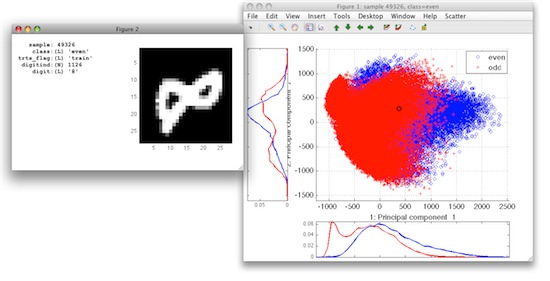
29.3. Visualizing the data in scatter plot ↩
We perform PCA projection to 30D subspace and visualize MNist training set in the scatter plot:
>> p=sdpca(tr,30)
PCA pipeline              784x30  73% of variance

>> sdscatter(tr*p)

ans =

 1
In order to see the digit images corresponding to a data sample, we add the 'imsize' data property with image size to our data set:
>> tr=setprop(tr,'imsize',[28 28],'data')
60000 by 784 sddata, 2 classes: 'even'(29492) 'odd'(30508)
Open in the Sample inspector via the Scatter menu and enter tr as the
name of the data set you wish to use. Hovering over data samples, we can
now see more details on each digit including its image:
29.4. Performance of base classifiers ↩
When dealing with a new classification problem, the recommended best practice is to start with the simple classifiers.
Apart of classifier error, we also consider training and execution speed.
It's often useful to start with Fisher linear discriminant and simple
Gaussian discriminant such as sdquadratic:
>> tic; pf=sdfisher(tr*p), toc
sequential pipeline       30x1 'Fisher linear discriminant'
 1 LDA                    30x1
 2 Gaussian model          1x2  single cov.mat.
 3 Normalization           2x2
 4 Decision                2x1  weighting, 2 classes
Elapsed time is 1.242268 seconds.

>> sdtest(ts,p*pf)

ans =

0.1409


>> tic; pg=sdquadratic(tr*p), toc
sequential pipeline       30x1 'Quadratic discriminant'
 1 Gaussian model         30x2  full cov.mat.
 2 Normalization           2x2
 3 Decision                2x1  weighting, 2 classes
Elapsed time is 1.168480 seconds.
>> sdtest(ts,p*pg)

ans =

0.0696
From the above, we can conclude that linear classifier is not good enough and quadratic is delivering better accuracy. (Note, that multi-modal problem may be still linearly separable if our sub-classes get favorably positioned in the feature space!)
29.5. Gaussian mixture models ↩
Mixture models can handle more non-linearity in the data by modeling distribution of each class a set of Gaussians.
>> tic; pm=sdmixture(tr*p); toc
[class 'even' init:.......... 10 clusters EM:done  10 comp] [class 'odd' init:.......... 10 clusters EM:done  10 comp]
Elapsed time is 204.558124 seconds.
>> sdtest(ts,p*pm)

ans =

0.0271
A mixture yield much lower error than a quadratic classifier. This suggests we need more non-linearity.
Does it help to increase the number of mixture components per class?
>> tic; pm2=sdmixture(tr*p,20); toc
[class 'even'EM:done  20 comp] [class 'odd'EM:done  20 comp]
Elapsed time is 195.213376 seconds.
>> sdtest(ts,p*pm2)

ans =

0.0192

>> tic; pm3=sdmixture(tr*p,30); toc
[class 'even'EM:done  30 comp] [class 'odd'EM:done  30 comp]
Elapsed time is 298.151235 seconds.
>> sdtest(ts,p*pm4)

ans =

0.0172

>> tic; pm3=sdmixture(tr*p,40); toc
[class 'even'EM:done  40 comp] [class 'odd'EM:done  40 comp]
Elapsed time is 403.129218 seconds.
>> sdtest(ts,p*pm4)

ans =

0.0167
Yes! We have enough training data to train mixtures with few tens of components.
Execution speed of the best solution:
>> pall=p*pm3
sequential pipeline       784x1 'PCA+Mixture of Gaussians+Decision'
 1 PCA                   784x30 73%% of variance
 2 Mixture of Gaussians   30x2  80 components, full cov.mat.
 3 Decision                2x1  weighting, 2 classes
>> tic; out=ts2*pall; toc
Elapsed time is 0.986567 seconds.
29.6. Classifiers based on the nearest neighbor rule ↩
The nearest neighbor classifier is another method that is directly applicable to multi-modal problems.
Performance of k-NN is dependent on two factors, namely size of its
training set (number of prototypes) and neighborhood size k.
Let us quickly test the k-NN performance when using 5000 prototypes randomly selected per-class:
>> proto=randsubset(tr*p,5000)
10000 by 30 sddata, 2 classes: 'even'(5000) 'odd'(5000)
>> tic; pk=sdknn(proto), toc
sequential pipeline       30x1 '1-NN+Decision'
 1 1-NN                   30x2  10000 prototypes
 2 Decision                2x1  weighting, 2 classes
Elapsed time is 0.077459 seconds.
>> sdtest(ts2,p*pk)

ans =

0.0237
You can see that the training stage is nearly instantaneous as k-NN only stores the prototypes.
Does different k help?
>> pk(1).k=2
sequential pipeline       30x1 '2-NN+Decision'
 1 2-NN                   30x2  10000 prototypes
 2 Decision                2x1  weighting, 2 classes
>> sdtest(ts,p*pk)

ans =

0.0207

>> pk(1).k=3
sequential pipeline       30x1 '3-NN+Decision'
 1 3-NN                   30x2  10000 prototypes
 2 Decision                2x1  weighting, 2 classes
>> sdtest(ts,p*pk)

ans =

0.0194
Yes, slightly higher k improves performance as it removes
noise-sensitivity of the k=1 classifier.
What about increasing number of prototypes?
>> proto=randsubset(tr*p,20000)
40000 by 30 sddata, 2 classes: 'even'(20000) 'odd'(20000)

>> pk=sdknn(proto,3)
sequential pipeline       30x1 '3-NN+Decision'
 1 3-NN                   30x2  40000 prototypes
 2 Decision                2x1  weighting, 2 classes

>> sdtest(ts,p*pk)

ans =

0.0138
The execution speed of the complete classifier on 10000 test samples:
>> pall=p*pk
sequential pipeline       784x1 'PCA+3-NN+Decision'
 1 PCA                   784x30 73%% of variance
 2 3-NN                   30x2  40000 prototypes
 3 Decision                2x1  weighting, 2 classes
>> tic; dec=ts2*pall; toc
Elapsed time is 10.480316 seconds.
29.7. Neural network classifier ↩
We will also investigate performance of a neural network in the subspace. The key parameters are the number of units in the hidden layer and the number of training iterations:
>> tic; pn=sdneural(tr*p,'units',50,'iters',10000); toc
Elapsed time is 2863.658793 seconds.
>> sdtest(ts,p*pn)

ans =

0.0653

>> tic; pn2=sdneural(tr*p,'units',80,'iters',10000); toc
Elapsed time is 4263.876124 seconds.
>> sdtest(ts,p*pn)

ans =

0.0493

>> tic; pn3=sdneural(tr*p,'units',200,'iters',20000); toc
Elapsed time is 19163.963511 seconds.
>> sdtest(ts,p*pn3)

ans =

0.0326
We can see that the neural network with a single layer does not reach the low error rates.
Execution speed of the best network:
>> pall=p*pn3;
>> tic; out=ts2*pall; toc
Elapsed time is 0.227642 seconds.
29.8. Random forest classifier ↩
In the random forest classifier, we can change the number of trees:
>> sub=randsubset(tr,5000)
10000 by 784 sddata, 2 classes: 'even'(5000) 'odd'(5000)

 >> tic; pr1=sdrandforest(sub*p,100); toc
 ..........
 Elapsed time is 238.955504 seconds.
 >>
 >> sdtest(ts,p*pr1)

 ans =

 0.0432

>> tic; pr2=sdrandforest(sub*p,200); toc
..........
Elapsed time is 477.693967 seconds.
>> sdtest(ts,p*pr2)

ans =

0.0419
The random forest does improve with growing number of trees but does not yield better error than about 4%.
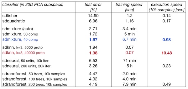
29.9. Summary table ↩
29.10. Conclusions ↩
We have seen how to choose a classifier for multi-modal problem. We started simple and gradually increased classifier complexity varying the major parameters.
We can conclude that:
The lowest error is reached by k-NN trained on a very large set of prototypes. This classifier is, however, quite slow in execution (11 sec per 10k samples)
Mixture of Gaussians also provides a low-error solution which is about 10 times faster in execution than k-NN (1 sec per 10k samples)
Neural networks and random forests did not reach low error solutions on this problem (using the 30D PCA subspace data representation)
Training time is lowest for the k-NN (instantaneous). Gaussian mixtures train on the 60000 samples in 30D in minutes. Neural nets and random forests requires tens of minutes. Dimensionality is the major bottleneck for neural net, training set size for the random forest.