Keywords: ROC analysis, output weighting, operating points

Given a two-class problem, with class names assigned as 'apple' and 'banana', we first divide the data set into a training set and a test set. This is important since the ROC analysis should always be performed on an independent set, i.e. on a set of samples unseen when learning the model.

>> load fruit; b=a(:,:,[1 2])
'Fruit set' 200 by 2 sddata, 2 classes: 'apple'(100) 'banana'(100) 
>> [tr,ts]=randsubset(b,0.5) 
'Fruit set' 100 by 2 sddata, 2 classes: 'apple'(50) 'banana'(50) 
'Fruit set' 100 by 2 sddata, 2 classes: 'apple'(50) 'banana'(50) 

We train a mixture of Gaussians on the training set, and apply the model to the test. The ROC for the two-class discriminant is estimated by weighting the two outputs of the disciminant. Finally, we visualize the ROC curve.

>> p=sdquadratic(tr);
sequential pipeline     2x2 'Quadratic discr.'
 1  Gauss full cov.         2x2  2 classes, 2 components (sdp_normal)
 2  Output normalization    2x2  (sdp_norm)
>> r=sdroc(ts*p)
ROC (2001 w-based op.points, 3 measures), curop: 1
est: 1:err(apple)=0.00, 2:err(banana)=0.02, 3:mean-error=0.01
>> sddrawroc(r)

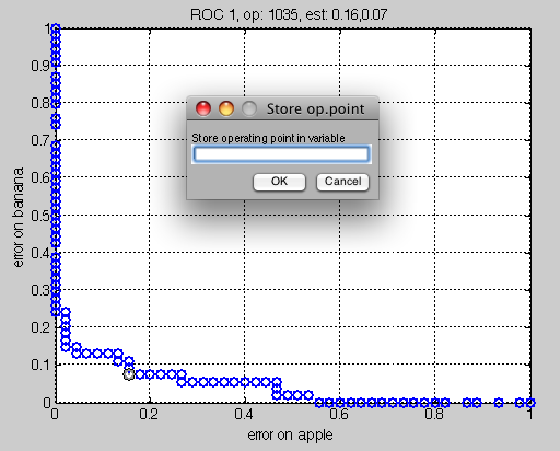
Press the s key (save) on the keyboard to store the selected operating point as default. A dialog will appear asking you to specify the variable name. We can, for example, enter r and store the operating point back to the ROC ob ject. Alternatively, the current operating point may be chosen as follows: r = setcurop(r,1035), (where 1035 is the index of the desired operating point). The following message in the Matlab promt will confirm the change in the settings.

Setting the operating point 1035 in sdroc object r
ROC (2001 w-based op.points, 3 measures), curop: 1035
est: 1:err(apple)=0.16, 2:err(banana)=0.07, 3:mean-error [0.50,0.50]=0.11

We can include the chosen operating point in the pipeline object. When applying the pipeline to new data c, the decision label are obtained for each new object.

>> pd = p*r
 sequential pipeline     2x1 'Quadratic discr.+Decision'
 1  Gauss full cov.         2x2  2 classes, 2 components (sdp_normal)
 2  Output normalization    2x2  (sdp_norm)
 3  Decision                2x1  weighting, 2 classes, ROC 2001 ops at op 1035 (sdp_decide)    
>> c=sddata(gendatf(15));  c=c(:,:,[1 2]); 
>> dec=c*pd;
>> +dec(1:5)

ans =

apple 
apple 
apple 
apple 
banana

Note that the data c can be a sddata object, or a simple raw matrix of numbers, with samples as rows and features as colums.