perClass Documentation
version 5.4 (7-Dec-2018)

Chapter 15: Classifier optimization with ROC Analysis

Table of contents

15.1. Introduction
15.2. Using sdroc objects

15.2.1. Setting current operating point
15.2.2. Performing decisions based on ROC
15.2.3. Interactive visualization of ROC decisions
15.2.4. Interactive visualization of confusion matrices
15.2.5. Defining constraints in a confusion matrix
15.2.6. Interactively minimizing errors in a confusion matrix
15.2.7. Accessing estimated performances
15.2.8. Using different performance measures

15.3. Multi-class ROC Analysis
15.4. ROC Analysis using target thresholding (detection)
15.5. Selecting application-specific operating point

15.5.1. The most common use-case
15.5.2. Applying performance constraints
15.5.3. Constraints using the low-level methods
15.5.4. Cost-sensitive optimization
15.5.5. Applying multiple performance constraints

15.6. Estimating ROC with variances

15.1. Introduction ↩

A trained classifier in perClass provides decisions by default. However, the default setting may not be ideal for our application. In this chapter, we will learn how to use a powerful tool helping us to find desirable operating points in our applications: The ROC analysis.

ROC abbreviation stands for the Receiver Operating Characteristic.

The basic idea of ROC analysis is very simple: For a given trained classifier and a labeled test set, define a set of possible operating points and estimate different type of errors at these points.

To optimize our classifier, we will need the following:

a trained classifier capable of returning soft outputs
knowledge of the soft outputs type (similarity or distance)
a labeled test set

ROC analysis works in three steps:

define admissible operating points
measure classifier performance at these points
select an operating point of interest based on application requirements

Let us consider a two-class problem with apple and banana classes. We will select the two classes of interest (data set a contains also the third class with outliers called stone).

>> load fruit; b=a(:,:,[1 2]);
>> [tr,ts]=randsubset(b,0.5) %  split the data into training and test set
'Fruit set' 100 by 2 sddata, 2 classes: 'apple'(50) 'banana'(50) 
'Fruit set' 100 by 2 sddata, 2 classes: 'apple'(50) 'banana'(50)

We train our classifier on the training set. We use the Fisher classifier:

>> p=sdfisher(tr)
sequential pipeline       2x1 'Fisher linear discriminant'
1 LDA                     2x1 
2 Gaussian model          1x2  single cov.mat.
3 Normalization           2x2 
4 Decision                2x1  weighting, 2 classes

Now we can estimate soft outputs of the Fisher classifier on the test set. We use -p to remove the classifier decision step and return the posterior probabilities for the two classes, i.e. the confidence that the sample belong to the class:

>> out=ts * -p
'Fruit set' 100 by 2 sddata, 2 classes: 'apple'(50) 'banana'(50)

The two outputs in out represent our two classes:

>> out.lab.list
sdlist (2 entries)
 ind name
   1 apple 
   2 banana

On the soft outputs, we perform ROC analysis using the sdroc command:

>> r=sdroc(out)
ROC (2001 w-based op.points, 3 measures), curop: 1042
est: 1:err(apple)=0.01, 2:err(banana)=0.04, 3:mean-error=0.02

sdroc defined a set of operating points, estimated three error measures (error on each class and the mean error), and fixed the "current" operating point to minimize the mean error.

An alternative syntax is to provide test set and a trained classifier instead of soft outputs:

>> r=sdroc(ts,p)
ROC (2001 w-based op.points, 3 measures), curop: 1042
est: 1:err(apple)=0.01, 2:err(banana)=0.04, 3:mean-error=0.02

We may visualize the ROC using the sddrawroc command:

>> sddrawroc(r)

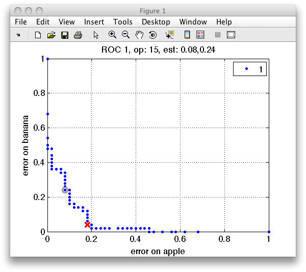
The ROC plot shows the first two measures in r, namely the error on apple class on the horizontal axis and the error on banana on the vertical axis. In the ROC plot, each blue marker represents one operating point. The current operating point is denoted by the red marker. When moving over the plot, the gray cursor marker follows the closest operating point. The figure title then shows the number of the cursor operating point and the values of the errors.

Note that selecting an operating point is a matter of trade-off. When we try to minimize error on one class, the error on the other at some moment inevitably increases. Only in the situation without class overlap, we could select an optimal solution. In real-world pattern recognition projects, we do need to accept certain level of errors. ROC analysis allows us to carefully choose the acceptable trade-off.

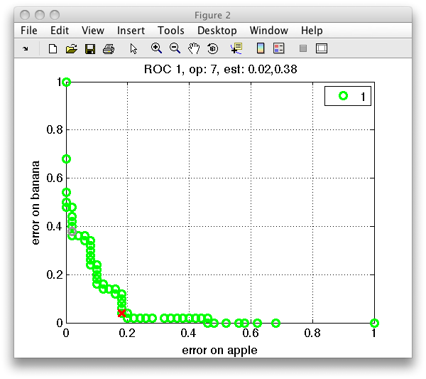
The ROC plot maybe customized with colors and markers as the standard Matlab plot. Simply add the chosen selection as a string in the second input:

>> sddrawroc(r,'go')

15.2. Using sdroc objects ↩

15.2.1. Setting current operating point ↩

Each ROC object has one operating point set as "current". The current operating point may be fixed interactively in the sddrawroc figure by clicking the left mouse button. By pressing the s key (save), we may store the current operating point index back to the sdroc object in the Matlab workspace. A dialog will open where we can specify the name sdroc variable or pipeline with ROC.

TIP: In the input dialog, you can press TAB key to move to the OK key and press ENTER.

Alternatively, we may set the current operating point manually using the setcurop function on Matlab prompt. The easiest option is to directly provide operating point index (which you may see in the interactive plot).

>> r2=setcurop(r,208)
ROC (2001 w-based op.points, 3 measures), curop: 208
est: 1:err(apple)=0.12, 2:err(banana)=0.02, 3:mean-error=0.07

Instead of index, setcurop allows us to set current operating point by constraining one of the performance measures and minimizing/maximizing other measure:

>> p=sdparzen(a)
....sequential pipeline       2x1 'Parzen model+Decision'
 1 Parzen model            2x2  200 prototypes, h=0.6
 2 Decision                2x1  weighting, 2 classes

>> r=sdroc(a,p)
ROC (158 w-based op.points, 3 measures), curop: 81
est: 1:err(apple)=0.02, 2:err(banana)=0.01, 3:mean-error=0.01

>> r=setcurop(r,'constrain','err(apple)',0.01,'min','err(banana)')
ROC (158 w-based op.points, 3 measures), curop: 78
est: 1:err(apple)=0.01, 2:err(banana)=0.04, 3:mean-error=0.03

More details in the section on application-specific setting of operating points.

15.2.2. Performing decisions based on ROC ↩

The sdroc object may be directly concatenated with the model pipeline via the * operator. This will add the decision action with all the ROC operating points:

>> pall=p*r
sequential pipeline       2x1 'LDA+Gaussian model+Normalization+Decision'
 1 LDA                     2x1 
 2 Gaussian model          1x2  single cov.mat.
 3 Normalization           2x2 
 4 Decision                2x1  ROC weighting, 2 classes, 2001 op.points at current 1042

The pd pipeline returns decisions at the current operating point:

>> sdconfmat(ts.lab,ts*pd)

ans =

 True      | Decisions
 Labels    | apple  banana  | Totals
-------------------------------------
 apple     |   165      1   |   166
 banana    |     7    159   |   166
-------------------------------------
 Totals    |   172    160   |   332

To relate the confusion matrix to the error measures in the ROC object, we may better use error normalization:

>> sdconfmat(ts.lab,ts*pd,'norm')

ans =

 True      | Decisions
 Labels    | apple  banana  | Totals
-------------------------------------
 apple     | 0.994  0.006   | 1.00
 banana    | 0.042  0.958   | 1.00
-------------------------------------

>> r
ROC (2001 w-based op.points, 3 measures), curop: 1042
est: 1:err(apple)=0.01, 2:err(banana)=0.04, 3:mean-error [0.50,0.50]=0.02

You can see that the error on apple class was 0.6% (rounded to 1% in the sdroc display above) and the error on the banana class 4.2%.

The confusion matrix at the ROC r2 with manually selected op.point 208:

>> sdconfmat(ts.lab,ts*p*r2,'norm')

ans =

 True      | Decisions
 Labels    | apple  banana  | Totals
-------------------------------------
 apple     | 0.880  0.120   | 1.00
 banana    | 0.024  0.976   | 1.00
-------------------------------------

15.2.3. Interactive visualization of ROC decisions ↩

We may visualize the ROC decisions at different operating points using the sdscatter command. We can connect the sdscatter to an open ROC figure. We only need to supply the data, the pipeline including the ROC operating points, and the number of the open ROC figure:

>> sdscatter(tr,p*r2,1)

We can now change the operating points in the ROC figure and directly observe the changes to the classifier decisions.

We can also open both plots in one step simply providing the ROC object to the sdscatter:

>> sdscatter(tr,p*r2,'roc')

15.2.4. Interactive visualization of confusion matrices ↩

sddrawroc is able to interactively visualize confusion matrices at different operating points. The advantage of this approach is that it is applicable to arbitrary problems, while the visualization of decisions is valid only for 2D feature spaces.

However, sdroc does not store confusion matrices by default. It only stores the desired performance measures. We must, therefore, add the confmat option when estimating the ROC:

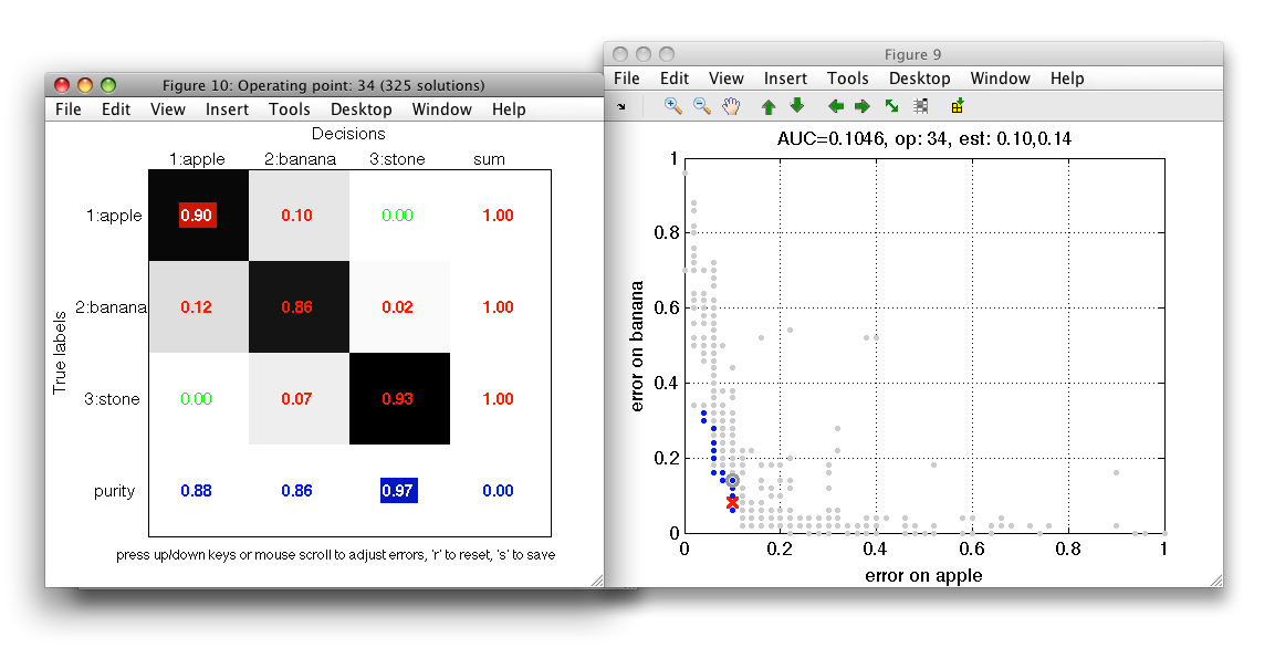
>> r=sdroc(a,p,'confmat')
ROC (124 w-based op.points, 3 measures), curop: 62
est: 1:err(apple)=0.09, 2:err(banana)=0.09, 3:mean-error=0.09

>> sddrawroc(r)

To open the confusion matrix window, press c in the ROC figure.

Visualizing confusion matrix for specific operating point in ROC analysis

The confusion matrix is opened in a separate figure. To view normalized confusion matrix, use 'n' key.

15.2.5. Defining constraints in a confusion matrix ↩

We may define performance constraints directly in the confusion matrix by clicking on its entries. We may constrain errors, performances and also the per-decision precision in the last row. When an entry is clicked, the ROC figure gets updated and rejected operating points are disabled. When moving mouse over the ROC plot, only the admissible entries are considered. This allows us to quickly inspect solution subsets given multiple constraints.

Interactive confusion matrix with multiple constraints showing multi-class ROC curve

The constrain value is remembered and applied even if the confusion matrix content is updated. This may happen when user moves the mouse over the connected ROC plot or by interactively lowering errors in the confusion matrix (see next section). The actual value in the error field cannot get above the original constrained error. Clicking a constrained field again disables the constrain.

15.2.6. Interactively minimizing errors in a confusion matrix ↩

Interactive confusion matrix allows us to directly minimize errors or maximize performances. We may do so by pointing mouse to a specific field with non-zero value and using a mouse scroll-wheel or up/down cursor keys. Confusion matrix will show a new cost-optimized solution. Note, that selected operating point in the ROC figure (red cross marker) will move acordingly.

Combination of constrains and interactive cost optimization in confusion matrix allows us to quickly explore possible solutions in a multi-class problem and find best trade-off.

15.2.7. Accessing estimated performances ↩

sdroc object behaves like a matrix with rows representing the operating points and columns the estimated performance measures. The order of columns is shown in the sdroc display string. We can extract performance estimates simply by addressing the sdroc as a matrix:

>> r2
ROC (2001 w-based op.points, 3 measures), curop: 208
est: 1:err(apple)=0.12, 2:err(banana)=0.02, 3:mean-error [0.50,0.50]=0.07
>> r2(206:208,:)

ans =

0.1205    0.0120    0.0663
0.1205    0.0181    0.0693
0.1205    0.0241    0.0723

The performance measures may be requested also by name:

>> r2(1:5,'err(apple)')

ans =

0.0120
1.0000
0.4759
0.4398
0.4157

The access to performance estimates is useful for custom selection of an operating point using application constraints.

15.2.8. Using different performance measures ↩

We may specify the performance measures used by sdroc command using the measures option. It takes a cell array with the list of desired measures. In this example, we will estimate commonly used ROC using true positive and false positive ratios:

>> load fruit; a=a(:,:,[1 2])
>> [tr,ts]=randsubset(a,0.5)
'Fruit set' 100 by 2 sddata, 2 classes: 'apple'(50) 'banana'(50) 
'Fruit set' 100 by 2 sddata, 2 classes: 'apple'(50) 'banana'(50)
>> p=sdnmean(tr) 
Nearest mean pipeline   2x2  2 classes, 2 components (sdp_normal)
>> out=ts*-p
'Fruit set' 100 by 2 sddata, 2 classes: 'apple'(50) 'banana'(50)
>> r=sdroc(out,'measures',{'FPr','apple','TPr','apple'})
ROC (2001 w-based op.points, 3 measures), curop: 1192
est: 1:FPr(apple)=0.14, 2:TPr(apple)=0.79, 3:mean-error=0.17
>> sddrawroc(r)

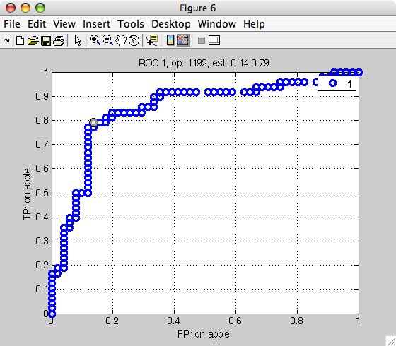
Note that in the measures option, we specify the measure name (FPr) followed by the class name. This is needed because the false positive rate depends on the definition of the target class. Because we specify the target is apple, the FPr is the error on banana misclassified as apple.

The following performance measures are supported:

mean-error: mean error over classes (default use equal class priors), optional parameter: vector with priors
class-errors: per class errors for each class
err: error of a specific class, parameter: name of class
TP, FP, FN, TN : e.g. TP = number of true positives, parameter: name of target class
TPr, FPr, FNr, TNr : e.g. TPr = true positive rate, parameter: name of target class
sensitivity, specificity, parameter: name of target class
precision : ratio of true positives in all positives TP/(TP+FP), parameter: name of target class
positive-fraction (posfrac): ratio of all positive decisions from all decisions (TP+FP)/N, parameter: name of target class
confmat : arbitrary entry of the confusion matrix, parameters: true class, decision, example: {'confmat','apple','banana'}
frac : fraction of given decisions from all samples (used for reject curves), parameter: decision of interest

All measures are also available for multi-class ROC. Non-targets are then defined as sum of all remaining classes.

15.3. Multi-class ROC Analysis ↩

In full generality, multi-class ROC has exponential complexity with respect to number of classes. However, practical sub-optimal solutions may be found using different search strategies. perClass allows us to perform multi-class ROC analysis using a greedy optimizer. Similarly to the two-class case, we simply pass the data with the model soft outputs to the sdroc command:

>> load eight_class
>> a
'Eight-class' 20000 by 2 sddata, 8 classes: [2468  2454  2530  2485  2530  2516  2502  2515]

>> a=randsubset(a,1000)
Multi-Class Problem, 1000 by 2 sddata, 8 classes: [130  110  111  145  116  119  137  132]
>> [tr,ts]=randsubset(a,0.5) 
Multi-Class Problem, 502 by 2 sddata, 8 classes: [65  55  56  73  58  60  69  66]
Multi-Class Problem, 498 by 2 sddata, 8 classes: [65  55  55  72  58  59  68  66]

>> p=sdmixture(tr,'comp',1,'iter',10)
[class 'a' EM:.......... 1 comp] [class 'b' EM:.......... 1 comp] 
[class 'c' EM:.......... 1 comp] [class 'd' EM:.......... 1 comp] 
[class 'e' EM:.......... 1 comp] [class 'f' EM:.......... 1 comp] 
[class 'g' EM:.......... 1 comp] [class 'h' EM:.......... 1 comp] 
Mixture of Gaussians pipeline 2x8  8 classes, 8 components (sdp_normal)          
>> out=ts*-p
Multi-Class Problem, 498 by 8 dataset with 8 classes: [65  55  55  72  58  59  68  66]
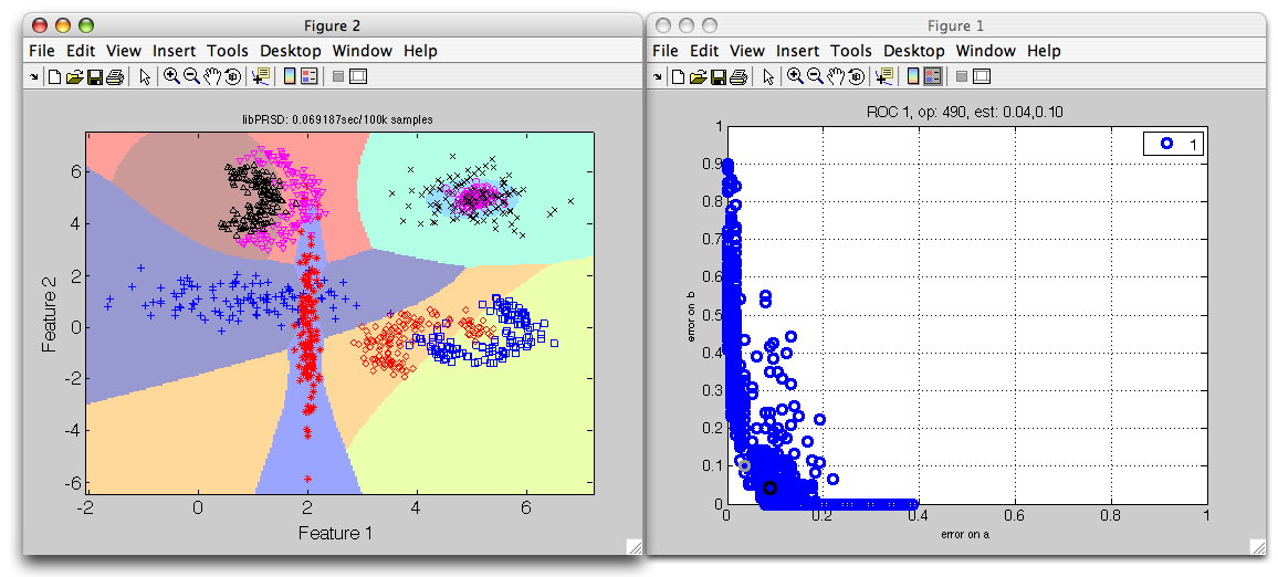
>> r=sdroc(out)
..........
ROC (2000 w-based op.points, 9 measures), curop: 318
est: 1:err(a)=0.12, 2:err(b)=0.04, 3:err(c)=0.02, 4:err(d)=0.42, 5:err(e)=0.02, 6:err(f)=0.00, 7:err(g)=0.03, 8:err(h)=0.03, 9:mean-error [0.12,0.12,...]=0.08
>> sdscatter(ts,p*r,'roc',r) %  visualize the scatter and ROC plot

>> load eight_class
>> a=randsubset(a,1000)
'Eight-class' 8000 by 2 sddata, 8 classes: [1000  1000  1000  1000  1000  1000  1000  1000]

>> [tr,ts]=randsubset(a,0.5) 
'Eight-class' 4000 by 2 sddata, 8 classes: [500  500  500  500  500  500  500  500]
'Eight-class' 4000 by 2 sddata, 8 classes: [500  500  500  500  500  500  500  500]

>> p=sdmixture(tr)
[class 'a' init:.......... 3 clusters EM:done  3 comp] [class 'b' init:.......... 4 clusters EM:done  4 comp] 
[class 'c' init:.......... 4 clusters EM:done  4 comp] [class 'd' init:.......... 1 cluster EM:done  1 comp] 
[class 'e' init:.......... 4 clusters EM:done  4 comp] [class 'f' init:.......... 4 clusters EM:done  4 comp] 
[class 'g' init:.......... 3 clusters EM:done  3 comp] [class 'h' init:.......... 3 clusters EM:done  3 comp] 
sequential pipeline       2x1 'Mixture of Gaussians+Decision'
 1 Mixture of Gaussians    2x8  26 components, full cov.mat.
 2 Decision                8x1  weighting, 8 classes

>> r=sdroc(ts,p)
..........
ROC (2000 w-based op.points, 9 measures), curop: 1
est: 1:err(a)=0.07, 2:err(b)=0.07, 3:err(c)=0.11, 4:err(d)=0.24, 5:err(e)=0.03, 6:err(f)=0.03, 7:err(g)=0.05, 8:err(h)=0.04, 9:mean-error=0.08
>> sub=randsubset(ts,100)
'Eight-class' 800 by 2 sddata, 8 classes: [100  100  100  100  100  100  100  100]
>> sdscatter(sub,p*r,'roc')

Note that you can switch between class errors shown the the ROC plot using the cursor keys (left/right for horizontal and up/down for vertical axis).

15.4. ROC Analysis using target thresholding (detection) ↩

In this section, we illustrate how to build ROC in target detection setting. This is achieved by thresholding the output of a model trained on a single (target) class.

Let us, for example, consider the problem where we want to detect all fruit in our fruit data set which contains apple and banana fruit examples and some stone (outlier) examples.

>> load fruit_large
>> a
'Fruit set' 2000 by 2 sddata, 3 classes: 'apple'(667) 'banana'(667) 'stone'(666) 

>> sub=randsubset(a,0.5)
'Fruit set' 999 by 2 sddata, 3 classes: 'apple'(333) 'banana'(333) 'stone'(333)

We will first create a two-class data set labeling all non-stone classes as fruit.

>> b=sdrelab(a,{'~stone','fruit'})
new lablist:
1: apple  -> fruit 
2: banana -> fruit 
3: stone  -> stone 
'Fruit set', 1000 by 2 sddata, 2 classes:  'stone'(334) 'fruit'(666) 

>> [tr,ts]=randsubset(b,0.5) %  split the data into training and validation
'Fruit set', 500 by 2 sddata, 2 classes: 'stone'(333)  'fruit' (167)
'Fruit set', 500 by 2 sddata, 2 classes: 'stone'(333)  'fruit' (167)

We will train a mixture model on the fruit class only:

>> p=sdmixture(data2(:,:,'fruit'),10)
[class 'fruit'EM:done  10 comp] 
sequential pipeline       2x1 'Mixture of Gaussians+Decision'
 1 Mixture of Gaussians    2x1  10 components, full cov.mat.
 2 Decision                1x1  threshold on 'fruit'

We will estimate soft outputs on our test set:

>> out=ts*-p
'Fruit set' 500 by 1 sddata, 2 classes: 'stone'(167) 'fruit'(333)

The out data contains one column representing the fruit class and contains labels of two classes (we need non-target examples to perform ROC):

>> out.featlab.list
sdlist (1 entries)
 ind name
   1 fruit
>> out.lab.list
sdlist (2 entries)
 ind name
   1 stone 
   2 fruit

The ROC analysis is straightforward:

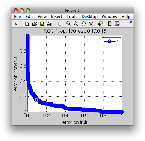
>> r=sdrocsdroc(out)
  1: stone  -> non-fruit
  2: fruit  -> fruit
ROC (500 thr-based op.points, 3 measures), curop: 170
est: 1:err(fruit)=0.10, 2:err(non-fruit)=0.16, 3:mean-error=0.13

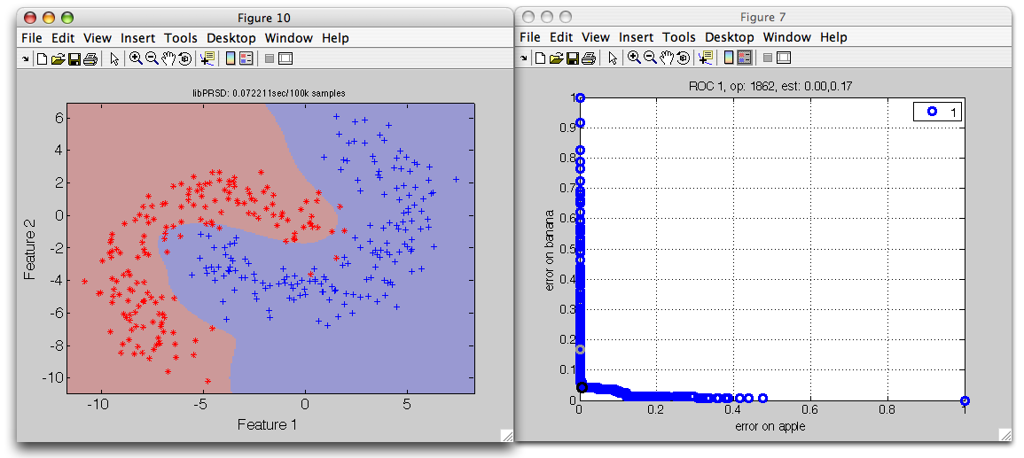
We visualize the detector decisions plotting the data a with all three classes:

>> sdscatter(a,p*r,'roc')

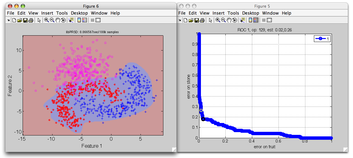
By thresholding the fruit model output, we effectively reject outliers.

15.5. Selecting application-specific operating point ↩

In our projects, we usually need to fix the operating point based on specific performance requirements. Two most common techniques are:

Common technique is to apply one or more performance constraints and then select an operating point by specific criteria. This may involve maximization of certain performance measure or minimizing total loss. The last approach is referred to as cost-sensitive optimization.

Applying performance constraints
Cost-sensitive optimization

15.5.1. The most common use-case ↩

The most common approach is to constrain one measure and fix the operating point by minimizing or maximizing other measure. This can be quickly achieved using setcurop method. In this example, we want to detect 99% of apples and minimize false positives:

>> p=sdparzen(a)
....sequential pipeline       2x1 'Parzen model+Decision'
 1 Parzen model            2x2  200 prototypes, h=0.6
 2 Decision                2x1  weighting, 2 classes

>> r=sdroc(a,p,'measures',{'TPr','apple','FPr','apple'})
ROC (124 w-based op.points, 3 measures), curop: 61
est: 1:TPr(apple)=0.91, 2:FPr(apple)=0.09, 3:mean-error=0.09

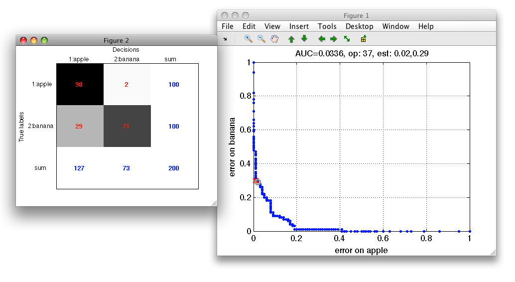
>> r=setcurop(r,'constrain','TPr(apple)',0.99,'min','FPr(apple)')
ROC (124 w-based op.points, 3 measures), curop: 89
est: 1:TPr(apple)=0.99, 2:FPr(apple)=0.30, 3:mean-error=0.15

We can observe, that if we find 99% of apples, our classifier returns 30% of false positives (bananas misclassified as apples).

15.5.2. Applying performance constraints ↩

Typically, we know specific constraints for our problem. For example, the maximum error on fruit may not exceed 10%.

We may apply performance constraints using the constrain method. It takes existing ROC object, specification of a performance measure (by its index or by name) and the constrain value.

Let us, for example, select subset of operating points with error on fruit lower than 20%:

>> r2=constrain(r,'err(fruit)',0.2)
ROC (216 thr-based op.points, 3 measures), curop: 170
est: 1:err(fruit)=0.10, 2:err(non-fruit)=0.16, 3:mean-error=0.13

This results in a subset of 216 operating points from the original 500. In this subset, the constrain method sets the current operating point minimizing the mean error over classes. We may be, however, interested in a different point, simply minimizing the error on the non-fruit. To do that, we can use the setcurop method:

>> r2=setcurop(r2,'min','err(non-fruit)')
ROC (216 thr-based op.points, 3 measures), curop: 212
est: 1:err(fruit)=0.19, 2:err(non-fruit)=0.11, 3:mean-error=0.15

Note that we ma reach 5% better error on non-fruit at the expense of higher mean error.

15.5.3. Constraints using the low-level methods ↩

We may also can apply constraints simply by querying the estimated performances in the ROC object using the standard Matlab commands such as find or min:

>> r
ROC (500 thr-based op.points, 3 measures), curop: 170
est: 1:err(fruit)=0.10, 2:err(non-fruit)=0.16, 3:mean-error=0.13

We will first find indices of all operating points with error on fruit smaller than 10%:

>> ind=find( r(:,'err(fruit)')<0.10 );

Now we can now find minimum error on non-fruit in this subset:

>> [m,ind2]=min( r(ind,'err(non-fruit)') );

And set the resulting operating point directly by the index:

>> r2=setcurop(r,ind(ind2))
ROC (500 thr-based op.points, 3 measures), curop: 170
est: 1:err(fruit)=0.10, 2:err(non-fruit)=0.16, 3:mean-error=0.13
>> sddrawroc(r2)

If criteria are too strict, the performance constraints may not be met. For example, if we wish not to exceed 10% error on fruit and 1% of stones, our classifier cannot provide a solution:

>> ind=find( r(:,'err(fruit)')<0.10 & r(:,'err(non-fruit)')<0.01 )

ind =

   Empty matrix: 0-by-1

15.5.4. Cost-sensitive optimization ↩

Second type of selecting operating point is based on an idea of misclassification costs. We can penalize different types of errors in confusion matrix and minimize classifier loss.

To perform cost-sensitive optimization, we need to fix our cost specification. This may come in a form of a cost matrix corresponding to the confusion matrix.

In this example, we will build a three-class mixture model for the fruit problem:

>> a
Fruit set, 1000 by 2 sddata, 3 classes: 'apple'(333) 'banana'(333) 'stone'(334) 
>> [tr,ts]=randsubset(a,0.5)
'Fruit set' 499 by 2 sddata, 3 classes: 'apple'(166) 'banana'(166) 'stone'(167) 
'Fruit set' 501 by 2 sddata, 3 classes: 'apple'(167) 'banana'(167) 'stone'(167) 
>> p=sdmixture(tr,'comp',[3 3 1],'iter',10)
[class 'apple' EM:.......... 3 comp] [class 'banana' EM:.......... 3 comp]
[class 'stone' EM:.......... 1 comp] 
sequential pipeline     2x3 ''
 1  sdp_normal          2x3  3 classes, 7 components

We can estimate the normalized confusion matrix at the default operating point:

>> sdconfmat(ts.lab,ts*sddecide(p),'norm')

ans =

 True      | Decisions
 Labels    | apple  banana stone   | Totals
--------------------------------------------
 apple     | 0.892  0.108  0.000   | 1.00
 banana    | 0.036  0.922  0.042   | 1.00
 stone     | 0.006  0.132  0.862   | 1.00
--------------------------------------------

We might be interested in lowering the fraction of apples misclassified as bananas. We will therefore specify the cost matrix in the following way:

>> m=ones(3); m(1,2)=5

m =

 1     5     1
 1     1     1
 1     1     1

Now we can perform ROC analysis using the cost-based optimization:

>> out=ts*-p
Fruit set, 499 by 3 sddata, 3 classes: 'apple'(166)  'banana'(166)  'stone'(167)
>> r=sdroc(out,'cost',m)
..........
ROC (100 w-based op.points, 4 measures), curop: 1
est: 1:err(apple)=0.01, 2:err(banana)=0.14, 3:err(stone)=0.14, 4:mean-error [0.33,0.33,...]=0.10

>> sdconfmat(ts.lab,ts*p*r,'norm')

ans =

 True      | Decisions
 Labels    | apple  banana stone   | Totals
--------------------------------------------
 apple     | 0.994  0.006  0.000   | 1.00
 banana    | 0.133  0.855  0.012   | 1.00
 stone     | 0.012  0.126  0.862   | 1.00
--------------------------------------------

The confusion matrix for the operating point found shows that we minimized the apple / banana error. Of course we pay in terms of banana / apple as each solution is a specific trade-off.

15.5.5. Applying multiple performance constraints ↩

Multiple performance constraints may be combined in one constrain call. Let us consider a multi-class ROC example where we try to optimize precision and per-class errors:

>> load fruit_huge
>> a
'Multi-Class Problem' 20000 by 2 sddata, 8 classes: [2468  2454  2530  2485  2530  2516  2502  2515]
>> [tr,ts]=randsubset(a,0.5) 
'Multi-Class Problem' 9999 by 2 sddata, 8 classes: [1234  1227  1265  1242  1265  1258  1251  1257]
'Multi-Class Problem' 10001 by 2 sddata, 8 classes: [1234  1227  1265  1243  1265  1258  1251  1258]

>> p=sdlinear(tr)
sequential pipeline     2x3 'Linear discriminant'
 1  Gauss eq.cov.           2x3  3 classes, 3 components (sdp_normal)
 2  Output normalization    3x3  (sdp_norm)

>> out=ts*-p
'Fruit set' 5001 by 3 sddata, 3 classes: 'apple'(1667) 'banana'(1667) 'stone'(1667) 

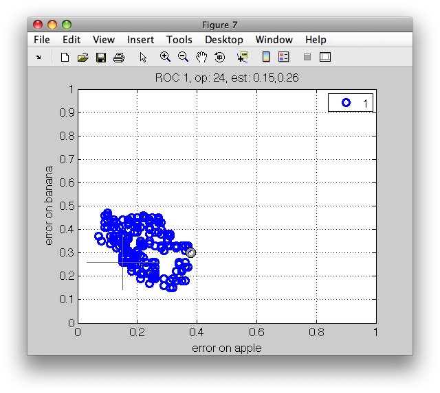
>> r=sdroc(out,'confmat','measures',{'precision','apple','class-errors'})
..........
ROC (2000 w-based op.points, 5 measures), curop: 1
est: 1:precision(apple)=0.84, 2:err(apple)=0.18, 3:err(banana)=0.23, 4:err(stone)=0.11, 5:mean-error=0.17

>> sddrawroc(r)

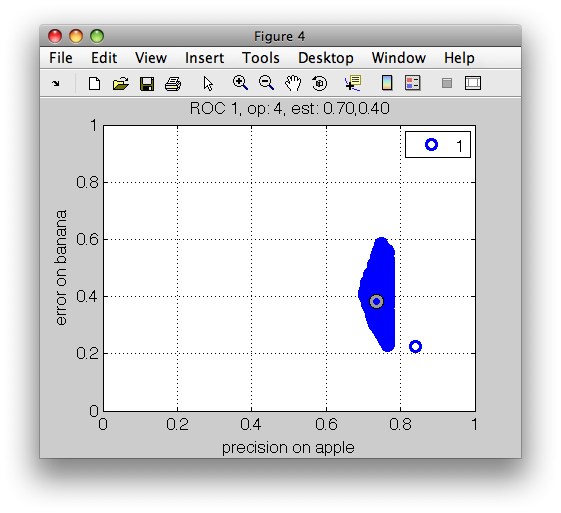
We are interested in precisions above 75% and banana errors under 30%:

>> r2=constrain(r,'precision(apple)',0.75,'err(banana)',0.3)
ROC (260 w-based op.points, 5 measures), curop: 1
est: 1:precision(apple)=0.84, 2:err(apple)=0.18, 3:err(banana)=0.23, 4:err(stone)=0.11, 5:mean-error=0.17

Remember that the oprating point is selected in this subset to minimize mean error. This default solution yields the following confusion matrix:

>> sdconfmat(ts.lab,out*r2)

ans =

 True      | Decisions
 Labels    |  apple banana  stone  | Totals
--------------------------------------------
 apple     |  1373    268     26   |  1667
 banana    |   236   1289    142   |  1667
 stone     |    27    153   1487   |  1667
--------------------------------------------
 Totals    |  1636   1710   1655   |  5001

We are, however, intrested in lowering the amount of apples, misclassified as bananas as apples are in our problem more costly. Therefore, we set the following cost matrix, penalizing this type of error with high cost:

>> m=ones(3); m(1,2)=10

m =

 1    10     1
 1     1     1
 1     1     1

We may now select the operating point in our subset minimizing the loss function considering our cost specification:

>> r2=setcurop(r2,'cost',m)
ROC (260 w-based op.points, 5 measures), curop: 4
est: 1:precision(apple)=0.75, 2:err(apple)=0.07, 3:err(banana)=0.29, 4:err(stone)=0.17, 5:mean-error=0.18

>> sdconfmat(ts.lab,out*r2)

ans =

 True      | Decisions
 Labels    |  apple banana  stone  | Totals
--------------------------------------------
 apple     |  1546    119      2   |  1667
 banana    |   413   1185     69   |  1667
 stone     |   101    184   1382   |  1667
--------------------------------------------
 Totals    |  2060   1488   1453   |  5001

The final classifier is composed of a model p with the operating point in r2:

>> pd=p*r2
sequential pipeline     2x1 'Linear discriminant+Decision'
 1  Gauss eq.cov.           2x3  3 classes, 3 components (sdp_normal)
 2  Output normalization    3x3  (sdp_norm)
 3  Decision                3x1  weighting, 3 classes, 260 ops at op 4 (sdp_decide)

15.6. Estimating ROC with variances ↩

ROC characteristic is a set of performance estimates computed at a set of operating points. Therefore, when cross-validating a model on a data set, we end up with multiple ROCs, one per each fold. It would be useful to accompany ROC estimated in cross-validation by mean and standard deviation for each operating point similarly to the standard point estimates such as mean classification error.

Estimating ROC with variances is not trivial as the characteristics computed on different test sets comprise different operating points (thresholds or weight vectors).

perClass implements operating point averaging algorithm which is a simple and straight-forward procedure for estimating ROC with variances based on the article:

Variance estimation for two-class and multi-class ROC analysis using operating point averaging. P. Paclik, C. Lai, J. Novovicova, R.P.W.Duin. Proc. of the 19th Int. Conf. on Pattern Recognition (ICPR2008, Tampa, USA, December 2008), IEEE Press, 2008.

The main idea is to estimate unbiased soft outputs of the model of interest using stacked generalization (cross-validation storing model soft outputs). ROC analysis on these soft outputs defines a single set of operating points. Going back to individual folds of the stacked generalization, we may estimate per-fold measures of interest at identical operating points. Eventually, we obtain their means and standard deviations over folds.

Let's illustrate the estimation of three-class ROC with variances:

>> load fruit_large
Fruit set, 2000 by 2 dataset with 3 classes: [667  667  666]

>> out=sdstackgen(sdnmean,a,'seed',42)
10 folds: ..........
'Fruit set' 2000 by 3 sddata, 3 classes: 'apple'(667) 'banana'(667) 'stone'(666) 

>> r=sdroc(out)
..........
ROC (2000 w-based op.points, 4 measures), curop: 1118
est: 1:err(apple)=0.18, 2:err(banana)=0.27, 3:err(stone)=0.11, 4:mean-error=0.19

>> [s,rv,e]=sdcrossval(sdnmean,a,'seed',42,'ops',r)
10 folds: [1: ] [2: ] [3: ] [4: ] [5: ] [6: ] [7: ] [8: ] [9: ] [10: ] 

s =

 10-fold rotation, ROC with variances, performance at op.point 671

 ind mean (std)  measure
   1 0.25 (0.05) error on apple
   2 0.20 (0.04) error on banana
   3 0.13 (0.04) error on stone
   4 0.20 (0.03) mean error over classes, priors [0.3,0.3,0.3]


ROC (2000 w-based op.points, 4 measures, 10 folds), curop: 671
est: 1:err(apple)=0.25(0.05), 2:err(banana)=0.20(0.04), 3:err(stone)=0.13(0.04), 4:mean-error=0.20(0.03)
completed 10-fold evaluation 'sde_rotation' (ppl: '')

The sdcrossval command returns string result summary, ROC object with per-fold estimated measures and evaluation object containing the per-fold trained classifiers.

sddrawroc shows the error-bars around the operating points.

>> sddrawroc(rv)

By pressing the 'f' key, sddrawroc displays the per-fold performances. This helps us to understand the worst-case misclassification scenario.