perClass Documentation
version 5.4 (7-Dec-2018)

Chapter 13.8: Decision trees and random forests

This section describes decision trees and random forest classifiers.

13.8.1. Decision tree classifier

13.8.1.1. Growing tree without pruning
13.8.1.2. Controlling the tree pruning
13.8.1.3. Using decision tree for feature selection

13.8.2. Random forest classifier

13.8.1. Decision tree classifier ↩

perClass sdtree classifier offers a fast and scalable decision tree implementation. Decision tree is build by finding the best threshold on one of the features that improves class separation. The process is applied recursively until the stopping condition is met. If the tree is fully built, each data sample ends in a separate terminal node. This solution, however, does not yield good generalization in case of class overlap. As with other classifiers, perClass strives to provide good solution by default. Therefore, sdtree applies pruning strategy that stops tree growth at the earlier stage. The pruning uses a separate validation set to estimate tree generalization error.

To illustrate the basic use of the decision tree, lets consider the fruit_large data set.

>> load fruit_large
>> a
'Fruit set' 2000 by 2 sddata, 3 classes: 'apple'(667) 'banana'(667) 'stone'(666)

We split the data to training and test subsets. The test subset will be used later to estimate tree performance.

>> [tr,ts]=randsubset(a,0.5)
'Fruit set' 999 by 2 sddata, 3 classes: 'apple'(333) 'banana'(333) 'stone'(333) 
'Fruit set' 1001 by 2 sddata, 3 classes: 'apple'(334) 'banana'(334) 'stone'(333)

We train the tree on the training subset tr. By default, the data set passed to sdtree is split internally into two subsets. The first part is used to grow the tree and the second part to limit its growth by identifying the sufficient number of thresholds. This process happens inside sdtree. We will see later, how to take closer control over the pruning process.

>> p=sdtree(tr)
sequential pipeline       2x1 'Decision tree'
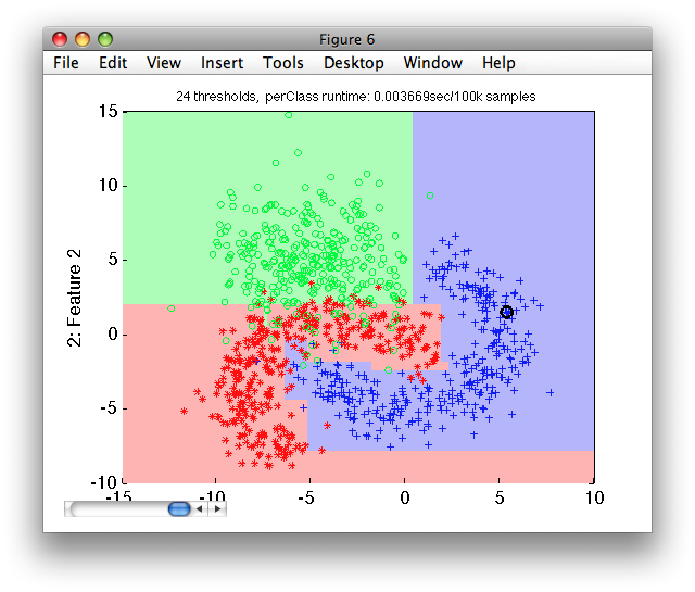
 1 Decision tree           2x3  14 thresholds on 2 features
 2 Decision                3x1  weighting, 3 classes

Let's visualize the decisions at the default operating point on the test set:

>> sdscatter(ts,p)

Default decision tree trained using sdtree.

We now estimate the mean test error using sdtest on the test subset:

>> sdtest(ts,p)

ans =

0.0779

13.8.1.1. Growing tree without pruning ↩

We may suppress the pruning process and grow the full tree, using the 'full' option.

>> p2=sdtree(tr,'full');
>> p2'
sequential pipeline     2x1 'Decision tree'
 1 Decision tree           2x3  97 thresholds on 2 features
       inlab: 'Feature 1','Feature 2'
         lab: 'apple','banana','stone'
      output: posterior
  thresholds: number of thresholds
        feat: features used
 2 Decision                3x1  weighting, 3 classes
       inlab: 'apple','banana','stone'
      output: decision ('apple','banana','stone')

Inspecting the pipeline steps, we can see that the number of thresholds and the features used are available for direct query. Note how the number of thresholds is much higher than when pruning the tree.

>>[p(1).thresholds p2(1).thresholds]

ans =

    14    97

We may compare the fully grown tree with the tree built using the default pruning strategy:

>> sdscatter(ts,p2)

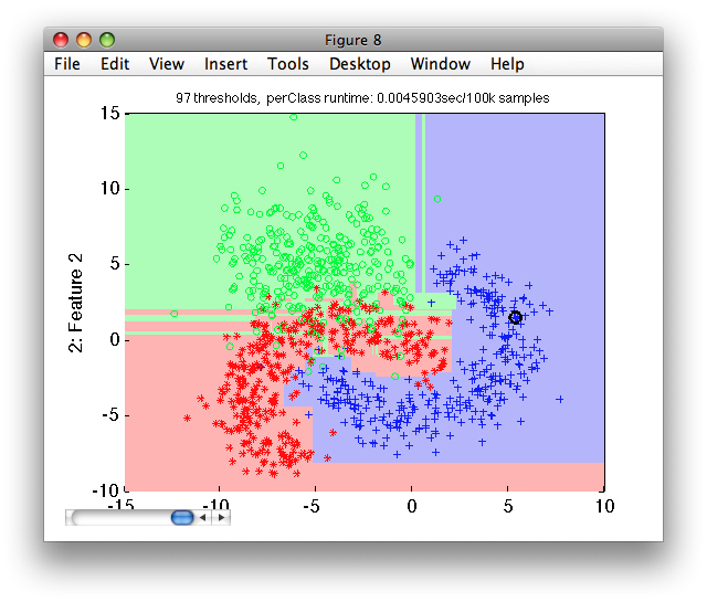
Fully-grown decision tree trained using sdtree.

Notice, the over-fitting appearing in the area of overlap. The fully-grown tree solves perfectly separates the training set but fails to do so on the independent test set.

13.8.1.2. Controlling the tree pruning ↩

We may control the sdtree pruning algorithm in several ways. Firstly, we may specify the fraction of the input data set used for training the tree using the 'trfrac' option. By default, 80% of input data is used to grow the tree and 20% to stop the growth process.

>> p=sdtree(tr,'trfrac',0.5)
sequential pipeline       2x1 'Decision tree'
 1 Decision tree           2x3  11 thresholds on 2 features
 2 Decision                3x1  weighting, 3 classes

Secondly, we may remove the random splitting step by supplying the separate validation data used for pruning.

>> [val,tr2]=randsubset(tr,100)
'Fruit set' 300 by 2 sddata, 3 classes: 'apple'(100) 'banana'(100) 'stone'(100) 
'Fruit set' 699 by 2 sddata, 3 classes: 'apple'(233) 'banana'(233) 'stone'(233)

We train on the tr2 part and pass the validation set val separately using the 'test' option:

>> p=sdtree(tr2,'test',val)
sequential pipeline       2x1 'Decision tree'
 1 Decision tree           2x3  11 thresholds on 2 features
 2 Decision                3x1  weighting, 3 classes

This removes the random element from the sdtree training. Repeating the training, we obtain identical tree.

>> p2=sdtree(tr2,'test',val)
sequential pipeline       2x1 'Decision tree'
 1 Decision tree           2x3  11 thresholds on 2 features
 2 Decision                3x1  weighting, 3 classes

>> [sdtest(ts,p) sdtest(ts,p2)]

ans =

    0.0829    0.0829

Thirdly, the number of tree levels (thresholds) may be also specified using the 'levels' option during the tree training:

>> p=sdtree(tr,'levels',10);
>> p(1).thresholds

ans = 

    10

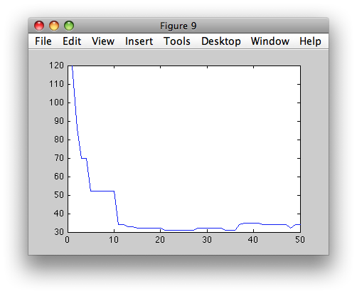
We may also inspect the pruning process in detail. The second output parameter, returned by sdtree, is a structure containing the full tree and the error criterion estimated from the validation set at each tree threshold.

>> [p,res]=sdtree(tr2,'test',val)
sequential pipeline       2x1 'Decision tree'
 1 Decision tree           2x3  11 thresholds on 2 features
 2 Decision                3x1  weighting, 3 classes

res = 

    full_tree: [2x3 sdppl]
          err: [42x1 int32]

>> figure; plot(res.err)

Error of the decision tree on the validation set.

The res.full_tree field contains the fully grown tree. To be more precise, it contains the tree grown as much as possible depending on the 'maxsamples' option. By default, at least 10 samples much be present in a node to continue growing process.

To prune the tree manually, we may select a specific number of thresholds by passing tree pipeline to the sdtree function. Here, we select 10 thresholds:

>> p3=sdtree(p,10)
sequential pipeline       2x1 'Decision tree+Decision'
 1 Decision tree           2x3  10 thresholds on 2 features
 2 Decision                3x1  weighting, 3 classes

13.8.1.3. Using decision tree for feature selection ↩

Decision trees optimize class separability considering all features. Therefore, a trained tree allows us to identify the features that provided most separability in our problem. In other words, we may use it for feature selection.

In this example, we train a tree classifier on medical data set:

>> a
'medical D/ND' 5762 by 10 sddata, 2 classes: 'disease'(1495) 'no-disease'(4267) 

>> p=sdtree(a)
sequential pipeline       10x1 'Decision tree'
1 Decision tree          10x2  41 thresholds on 8 features
2 Decision                2x1  weighting, 2 classes

You may see in the pipeline comment, that only 8 features form 10 is used in this tree. Removing the unused features allows us to limit the amount of computation we need in our final system.

By passing the tree to sdfeatsel function, we obtain a pipeline describing the same classifier but only on these 8 features:

>> pf=sdfeatsel(p)
sequential pipeline       10x1 'Feature subset+Decision tree+Decision'
1 Feature subset         10x8 
2 Decision tree           8x2  41 thresholds on 8 features
3 Decision                2x1  weighting, 2 classes

The first step in the pipeline pf is the feature selection. We may list the features that are useful:

>> +pf(1).lab

ans =

StdDev       
Skew         
Kurtosis     
Energy Band 1
Energy Band 2
Moment 20    
Moment 02    
Fractal 4

Typically, we would use this first step in the pipeline pf to create a new data set with only relevant features:

>> b=a*pf(1)
'medical D/ND' 5762 by 8 sddata, 2 classes: 'disease'(1495) 'no-disease'(4267)

The classifier pf(2:end) is running on this data set:

>> dec=b*pf(2:end)
sdlab with 5762 entries, 2 groups: 'disease'(1459) 'no-disease'(4303)

13.8.2. Random forest classifier ↩

Random forest classifier sdrandforest combines a large number of specifically-built decision trees. Each tree is built by considering only randomly selected subset of features at each tree node. The combination of their outputs is based on the sum rule.

By default, sdrandforest builds 20 trees and considers a subset of 20% of features at each node. Let us train a random forest classifier on the medical data set. We use data of the first five patients as a test set and remaining data as a training set:

>> load medical
>> a=a(:,:,1:2)
'medical D/ND' 5762 by 11 sddata, 2 classes: 'disease'(1495) 'no-disease'(4267) 
>> [ts,tr]=subset(a,'patient',1:5)
'medical D/ND' 1887 by 11 sddata, 2 classes: 'disease'(597) 'no-disease'(1290) 
'medical D/ND' 3875 by 11 sddata, 2 classes: 'disease'(898) 'no-disease'(2977) 

>> p=sdrandforest(tr)
..........
sequential pipeline       11x1 'Random forest+Decision'
 1 Random forest          11x2  20 trees
 2 Decision                2x1  weighting, 2 classes
>> sdtest(ts,p)

ans =

0.2730

sdrandforest offers several user-adjustable parameters. For example, we may alter the number of trees and the number of randomly-selected dimensions.

The number of trees may be provided directly as the second parameter:

>> p=sdrandforest(tr,200)
..........
sequential pipeline       11x1 'Random forest+Decision'
 1 Random forest          11x2  200 trees
 2 Decision                2x1  weighting, 2 classes
>> sdtest(ts,p)

ans =

0.2848

To adjust the number of dimensions that are randomly selected at each tree node during training, use the 'dim' option. Here we combine it with the request for the 200 trees:

>> p=sdrandforest(tr,'dim',0.5,'count',200)
..........
sequential pipeline       11x1 'Random forest+Decision'
 1 Random forest          11x2  200 trees
 2 Decision                2x1  weighting, 2 classes    

>> sdtest(ts,p)

ans =

0.2798