perClass Documentation
version 5.4 (7-Dec-2018)

Chapter 13.2: Gaussian models

This section describes perClass classifiers based on assumption of Gaussian distribution.

13.2.1. Introduction
13.2.2. Nearest mean classifier

13.2.2.1. Scaled nearest mean

13.2.3. Linear discriminant assuming normal densities
13.2.4. Quadratic classifier assuming normal densities
13.2.5. Gaussian model or classifier
13.2.6. Constructing Gaussian model from parameters
13.2.7. Generating data based on Gaussian model
13.2.8. Gaussian mixture models

13.2.8.1. Automatic estimation of number of mixture components
13.2.8.2. Choosing number of mixture components manually
13.2.8.3. Clustering data using a mixture model

13.2.9. Regularization of Gaussian models

13.2.1. Introduction ↩

The family of Gaussian classifiers assumes that the observations are generated by a random process that has normal distribution. Density function of a normal distribution is defined by mean vector, and covariance matrix. If multiple Gaussian models are used, they are additionally weighted by priors.

In the simplest situation, the assumption is that each class is defined by a single Gaussian density. This yields nearest mean, linear and quadratic classifier. More complex setup assumes that each class may be modeled by a mixture of several Gaussians. This results in Gaussian mixture models.

In general, classifiers based on assumption of normality estimate probability densities. Therefore, their use is in practice limited to lower-dimensional situations. If the number of samples is too low compared to dimensionality or data exhibit strong subspace structure, normal models have difficulties in inverting covariance matrices.

13.2.2. Nearest mean classifier ↩

The nearest mean classifier sdnmean leverages assumption of normality. It uses normal model with identity covariance matrix for all classes.

Nearest mean is one of the most simple classifiers useful in situations with few samples and large number of features.

>> load fruit
260 by 2 sddata, 3 classes: 'apple'(100) 'banana'(100) 'stone'(60) 
>> p=sdnmean(a)
sequential pipeline       2x1 'Nearest mean+Decision'
 1 Nearest mean            2x3  unit cov.mat.
 2 Decision                3x1  weighting, 3 classes
>> sdscatter(a,p)

Decision
boundary of the nearest mean classifier

An alternative formulation of nearest mean using distances to prototypes is described here.

As for all Gaussian models, user may provide apriori-known class prior probabilities when training sdnmean with 'priors' option. If not provided, priors are estimated from training data set.

13.2.2.1. Scaled nearest mean ↩

With the 'scaled' option, sdnmean uses covariance matrices with a separately estimated variance for each feature.

In this way, nearest mean classifier takes into account data scaling and will not change if the multiplicative scaling of features is applied.

>> p2=sdnmean(tr,'scaled')
sequential pipeline       2x1 'Nearest mean+Decision'
1 Nearest mean            2x3  scaled diag.cov.mat
2 Decision                3x1  weighting, 3 classes

13.2.3. Linear discriminant assuming normal densities ↩

sdlinear is a linear discriminant based on assumption of normal densities. The pooled covariance matrix is computed by averaging per-class covariances taking into account class priors.

>> load fruit;
>> a=a(:,:,[1 2])
260 by 2 sddata, 2 classes: 'apple'(100) 'banana'(100)  

>> p=sdlinear(a)
sequential pipeline       2x1 'Gaussian model+Normalization+Decision'
 1 Gaussian model          2x2  single cov.mat.
 2 Normalization           2x2 
 3 Decision                2x1  weighting, 2 classes

Note the normalization step in the pipeline p. This assures that the sdlinear soft output is posterior probability (confidence). Due to this normalization, sdlinear requires two or more classes be present in the input data set.

Confusion matrix estimated on the training set at default operating point:

>> sdconfmat(a.lab,a*p,'norm')

ans =

 True      | Decisions
 Labels    | apple  banana  | Totals
-------------------------------------
 apple     | 0.890  0.110   | 1.00
 banana    | 0.150  0.850   | 1.00
-------------------------------------

In order to use specific priors, provide them using the priors option:

>> p=sdlinear(a,'priors',[0.8 0.2])
sequential pipeline       2x1 'Gaussian model+Normalization+Decision'
 1 Gaussian model          2x2  single cov.mat.
 2 Normalization           2x2 
 3 Decision                2x1  weighting, 2 classes

>> sdconfmat(a.lab,a*p,'norm')

ans =

 True      | Decisions
 Labels    | apple  banana  | Totals
-------------------------------------
 apple     | 0.950  0.050   | 1.00
 banana    | 0.200  0.800   | 1.00
-------------------------------------

Note that by increasing the apple class prior we lower the apple error. However, the banana error will increase accordingly.

The sdlinear classifier may be regularized by adding a small constant to a covariance diagonal. See the following section for an example on how to use automatic regularization.

13.2.4. Quadratic classifier assuming normal densities ↩

sdquadratic implements quadratic discriminant based on assumption of normal densities. In fact, sdquadrartic is composed of an sdgauss pipeline with an extra normalization step that makes sure the classifier returns posteriors. Due to this class normalization, sdquadratic can only be trained on data set with two or more classes.

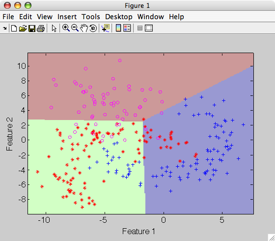
The quadratic decision boundary is achieved by estimating a specific covariance matrix for each class.

>> p=sdquadratic(a)
sequential pipeline       2x1 'Quadratic discriminant'
 1 Gaussian model          2x2  full cov.mat.
 2 Normalization           2x2 
 3 Decision                2x1  weighting, 2 classes

Detailed display of pipeline contents shows the outputs of the first and second step (density and posterior):

>> p'
sequential pipeline     2x1 'Quadratic discriminant'
 1 Gaussian model          2x3  full cov.mat.
   inlab: 'Feature 1','Feature 2'
     lab: 'apple','banana','stone'
  output: probability density
 complab: component labels
 2 Normalization           3x3 
   inlab: 'apple','banana','stone'
     lab: 'apple','banana','stone'
  output: posterior
 3 Decision                3x1  weighting, 3 classes
   inlab: 'apple','banana','stone'
  output: decision ('apple','banana','stone')

Visualizing the classifier decisions:

>> sdscatter(a,p)

Quadratic classifier assuming normal densities

Similarly to other normal-based models, the user may fix class priors with 'priors' option, if know apriori.

13.2.5. Gaussian model or classifier ↩

sdgauss implements a general Gaussian model or classifier with full covariances. By default, sdgauss returns a classifier:

>> p=sdgauss(a)
sequential pipeline       2x1 'Gaussian model+Decision'
1 Gaussian model          2x3  full cov.mat.
2 Decision                3x1  weighting, 3 classes

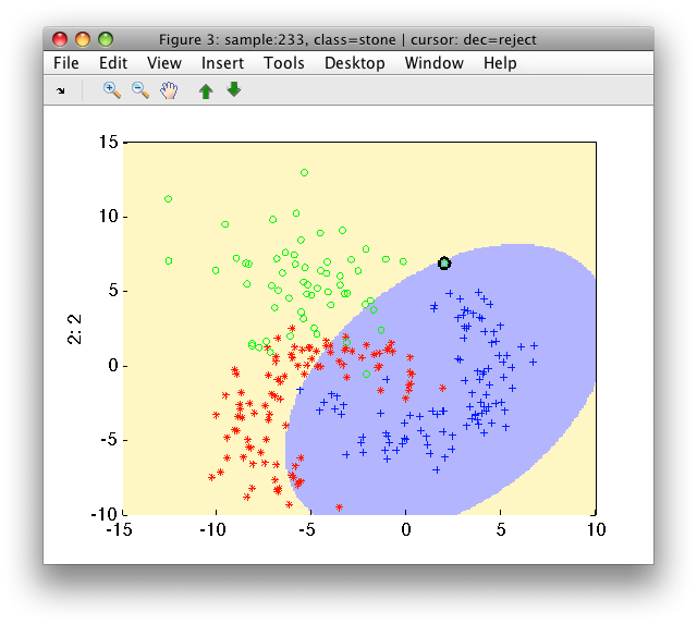
Unlike sdquadratic, sdgauss does not normalize class outputs. It returns probability density and, therefore, may be used to build a detector.

In fact, training sdgauss on data with only one class returns a one-class classifier that accepts all training examples:

>> a
'Fruit set' 260 by 2 sddata, 3 classes: 'apple'(100) 'banana'(100) 'stone'(60) 
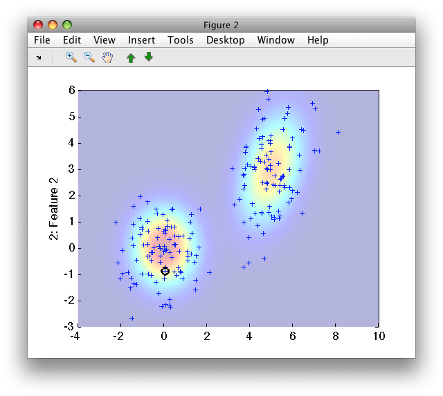
>> p=sdgauss(a(:,:,'apple'))
sequential pipeline       2x1 'Gaussian model+Decision'
1 Gaussian model          2x1  full cov.mat.
2 Decision                1x1  threshold on 'apple'
>> sdscatter(a,p)

Gaussian one-class detector accepting all target examples.

13.2.6. Constructing Gaussian model from parameters ↩

sdgauss may be also used to create Gaussian pipeline from parameters. We need to provide:

sddata set with component means
cell array with covariance matrices
vector of priors with an entry for each component

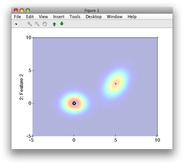
Example: I'd like to create a model with two components, one with mean at [0 0] and the other at [5 3] with the first covariance unit and second [1 0.3; -0.8 0.5].

>> m=sddata([0 0; 5 3])
2 by 2 sddata, class: 'unknown'
>> cov={eye(2) [1 .5; .5 2]}

cov = 

[2x2 double]    [2x2 double]

>> prior=[0.5 0.5]

prior =

0.5000    0.5000

>> p=sdgauss(m,cov,prior)
Gaussian model pipeline   2x1

To visualize the output of the pipline p, we need a data set to pass to sdscatter. We can use class means and add two points extending our view:

>> sdscatter(sddata([+m; -5 -5; 10 10]),p)

Density of a manually-defined Gaussian model

13.2.7. Generating data based on Gaussian model ↩

Gaussian model are "generative" which means we can use them to create a data set following the same distribution.

In perClass, we may use the sdgenerate command to do that. Using the pipeline p form the previous section, we can create data set with 100 samples per component by:

>> b=sdgenerate(p,100)
200 by 2 sddata, class: 'unknown'
>> sdscatter(b,p)

Generating random data from Gaussian model.

13.2.8. Gaussian mixture models ↩

Gaussian mixture is a density-estimation approach using a weighted sum of multiple Gaussian components. The sdmixture implements a classifier with a separate mixture model, estimated for each of the classes.

Advantage of a mixture classifier is its flexibility. Given enough training data, it may reliably model class distributions with arbitrary shapes or disjoint clusters (modes). Multi-modal data often originate in applications where our top-level classes reflect a composition of underlying states. For example, a medical diagnostic tool aims at detection of cancer. As the disease may affect different tissues, we observe our "cancer" class as a multi-modal composition of separate data tissue clusters. Mixture classifier can naturally describe such class distribution.

While parameters of a single Gaussian model may be estimated directly from data, mixture models require iterative optimization based on EM algorithm.

13.2.8.1. Automatic estimation of number of mixture components ↩

In perClass, the sdmixture command does not need any input arguments apart of training data:

>> a
'Fruit set' 260 by 2 sddata, 3 classes: 'apple'(100) 'banana'(100) 'stone'(60) 

>> p=sdmixture(a)
[class 'apple' init:.......... 4 clusters EM:done  4 comp] [class 'banana' init:....
...... 4 clusters EM:done  4 comp] [class 'stone' init:.......... 2 clusters EM:done  2 comp] 
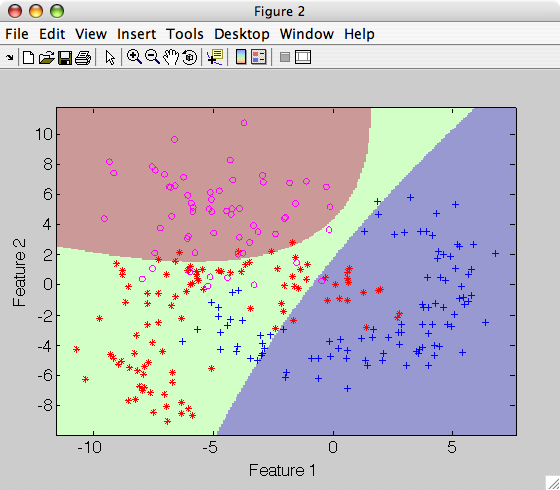
sequential pipeline       2x1 'Mixture of Gaussians+Decision'
1 Mixture of Gaussians    2x3  10 components, full cov.mat.
2 Decision                3x1  weighting, 3 classes

>> sdscatter(a,p)

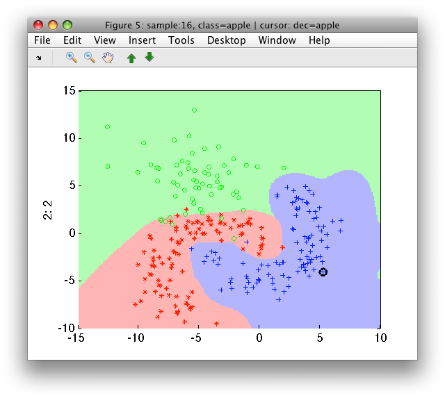
Decisions of a Gaussian mixture classifier automatically estimating number of components.

By default, sdmixture automatically identifies the number of components for each class and then estimates each per-class mixture running 100 iterations of EM algorithm. Number of iterations can be changed with 'iter' option.

The estimation of the number of components performs an internal random split of the input data set. Therefore, we will receive potentially different solution each run. Fixing the seed of the Matlab random number generator makes the sdmixture training repeatable.

>> rand('state',1234); p=sdmixture(a)  %  example of setting random seed

Let us visualize the soft outputs of the mixture. We will use -p shorthand to remove the decision step:

>> sdscatter(a,-p)

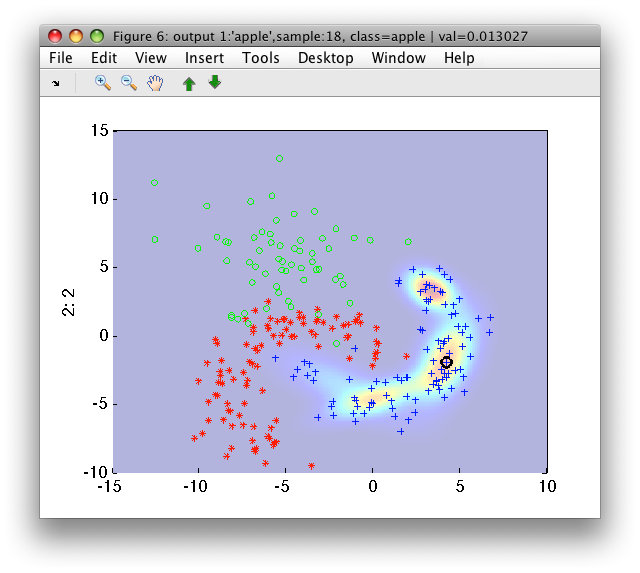
Soft outputs of a mixture classifier automatically estimating number of components.

We can see the density of the mixture model for the first class ('apple') comprised of four components. Clicking the arrow buttons on the Figure toolbar, we can see the density estimates for the second and third class

The estimation of number of components is performed on a subset of the input data. By default 500 samples is used per class. This may be adjusted using 'maxsamples' option.

The algorithm uses a grid search considering 1:10 clusters by default. The grid may be adjusted with 'cluster grid' option.

13.2.8.2. Choosing number of mixture components manually ↩

We may fix the number of mixture components manually by providing it as the second argument:

>> p=sdmixture(a,5)
[class 'apple'EM:done  5 comp] [class 'banana'EM:done  5 comp] [class 'stone'EM:done  5 comp] 
sequential pipeline       2x1 'Mixture of Gaussians+Decision'
1 Mixture of Gaussians    2x3  15 components, full cov.mat.
2 Decision                3x1  weighting, 3 classes

If a scalar value is given, the same number of components is used for all classes.

By providing a vector, we may fix different number of components per class. In our example, we know that the 'stone' class is unimodal:

>> p=sdmixture(a,[5 5 1])
[class 'apple'EM:done  5 comp] [class 'banana'EM:done  5 comp] [class 'stone'EM:done  1 comp] 
sequential pipeline       2x1 'Mixture of Gaussians+Decision'
1 Mixture of Gaussians    2x3  11 components, full cov.mat.
2 Decision                3x1  weighting, 3 classes

13.2.8.3. Clustering data using a mixture model ↩

Mixture model which estimates the number of clusters automatically is a powerful data description tool. We may use it to cluster a data set i.e. to identify its distinct modes.

Let us consider a data set b with only one class. We create it by removing class labels from fruit data set:

>> a
'Fruit set' 260 by 2 sddata, 3 classes: 'apple'(100) 'banana'(100) 'stone'(60) 
>> b=sddata(+a)
260 by 2 sddata, class: 'unknown'

Let us train a mixture model twice. First, without any option:

>> rand('state',10); pc1=sdmixture(b)
[class 'unknown' init:.......... 8 clusters EM:done  8 comp] 
sequential pipeline       2x1 'Mixture of Gaussians+Decision'
1 Mixture of Gaussians    2x1  8 components, full cov.mat.
2 Decision                1x1  threshold on 'unknown'

Second, with 'cluster' option:

>> rand('state',10); pc2=sdmixture(b,'cluster')
[class 'unknown' init:.......... 8 clusters EM:done  8 comp] 
sequential pipeline       2x1 'Mixture of Gaussians+Decision'
1 Mixture of Gaussians    2x8  8 components, full cov.mat.
2 Decision                8x1  weighting, 8 classes

The rand commands make sure both estimated mixtures are identical.

The only difference between pipeline pc1 and pc2 is in labeling of the mixture components.

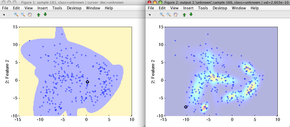
The mixture pc1 models all available data in b by one mixture model returning one soft output (see the output dimensionality of 1 in the pipeline step 1). Let us visualize the decisions and soft outputs of pc1:

>> sdscatter(b,pc1)

ans =

1

>> sdscatter(b,-pc1)

ans =

2

One-class mixture classifier.

The pc2 pipeline, trained with 'cluster' option, splits the complete mixture into individual components. Therefore, we can see 8 distinct soft output. Default decisions will be 'Cluster 1' to 'Cluster 8':

>> sdscatter(b,pc2)

ans =

3

>> sdscatter(b,-pc2)

ans =

4

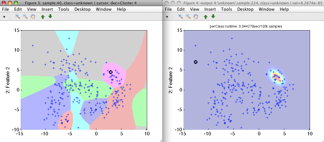
Clustering solution using a mixture model.

Note that we observe only one component at a time in the soft output Figure 4. Others are available via arrow buttons. The decisions of pc2 provide cluster labels.

13.2.9. Regularization of Gaussian models ↩

Regularization is a technique of avoiding problem with parameter estimation caused by with small number of data samples in a problem with large dimensionality.

Normal-based classifier suffer, in such situations, from low quality estimates of class covariances. This results either in poor classifier performance or failure to train on a given data set.

Possible solution is to add a small constant to diagonal elements of the covariance matrices. In perClass, this can be achieved with the 'reg' option.

In the following example, we want to recognize handwritten digits represented directly by pixels in 16x16 raster. Quadratic classifier fails to discriminate the digits if trained on our limited training set of 60 samples per class. The full covariances are not reliably estimated.

>> [tr,ts]=randsubset(a,0.3)
'Digits' 600 by 256 sddata, 10 classes: [60  60  60  60  60  60  60  60  60  60]
'Digits' 1400 by 256 sddata, 10 classes: [140  140  140  140  140  140  140  140  140  140]

>> p=sdquadratic(tr)
sequential pipeline       256x1 'Quadratic discriminant'
1 Gaussian model        256x10 full cov.mat.
2 Normalization          10x10
3 Decision               10x1  weighting, 10 classes
>> sdtest(ts,p)

ans =

0.9000

Using the 'reg' option, sdquadratic performs automatic choice of the regularization parameter. The test set error of the resulting classifier is only 8.5%!

>> p=sdquadratic(tr,'reg')
..........
 reg=0.100000 err=0.07
sequential pipeline       256x1 'Quadratic discriminant'
 1 Gaussian model        256x10 full cov.mat.
 2 Normalization          10x10
 3 Decision               10x1  weighting, 10 classes   

>> sdtest(ts,p)
ans =

 0.0921

The 'reg' option splits internally the provided data into two parts and performs a grid search. One part is used for training the model, the other one for evaluating the error. The default splitting fraction is 20% for validation. It may be changed with the 'tsfrac' option.

Alternatively, the internal splitting is avoided by providing the test (validation) set with 'test' option:

>> rand('state',42); [tr2,val]=randsubset(tr,0.5)
>> p=sdquadratic(tr2,'reg','test',val);

The regularization parameter may be provided directly:

>> p=sdquadratic(tr,'reg',0.01)