perClass Documentation
version 5.4 (7-Dec-2018)

Chapter 13.3: Gaussian models

This section describes classifiers based on k-th nearest neighbor rule.

13.3.1. k-NN classifier

13.3.2. Prototype selection for k-NN
13.3.3. k-means as a classifier

13.3.3.1. Adjusting number of centers in the k-means classifier
13.3.3.2. Changing k in the final k-NN classifier
13.3.3.3. Prototype pruning

13.3.1. k-NN classifier ↩

k-NN (k-th nearest neighbor) is a non-parametric classifier measuring distance between a new sample and stored "prototype" examples. Instead of building a model from training examples it uses them directly as evidence for computing its output on new observations.

By default sdknn implements the first nearest neighbor rule (k=1) using all provided training examples as prototypes:

>> load fruit
>> a
'Fruit set' 260 by 2 sddata, 3 classes: 'apple'(100) 'banana'(100) 'stone'(60) 

>> p=sdknn(a)
sequential pipeline       2x1 '1-NN+Decision'
1 1-NN                    2x3  260 prototypes
2 Decision                3x1  weighting, 3 classes
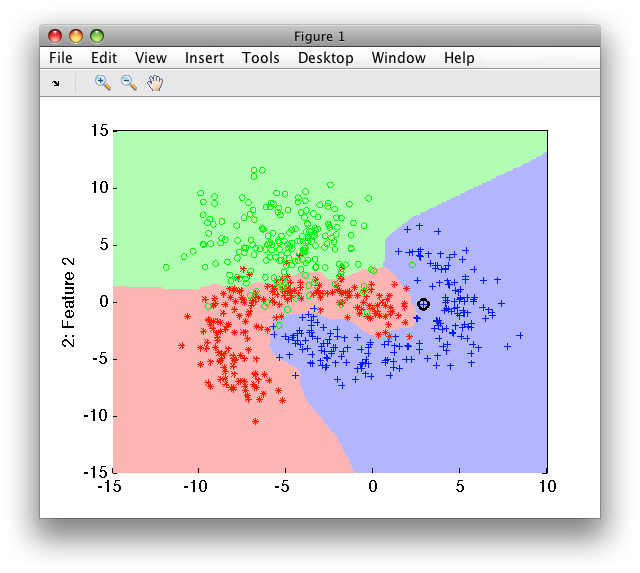
>> sdscatter(a,p)

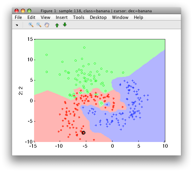
Using larger neighborhoods (k>1), the nearest neighbor classifier becomes more robust against noise in the areas of overlap.

13.3.1.1. Changing neighborhood size k ↩

We may specify the neighborhood size k as second parameter:

>> p3=sdknn(a,3)
sequential pipeline       2x1 '3-NN+Decision'
1 3-NN                    2x3  260 prototypes
2 Decision                3x1  weighting, 3 classes
>> sdscatter(a,p3)

An alternative is to directly change the k field in the pipeline step:

>> p3'
sequential pipeline     2x1 '3-NN+Decision'
 1 3-NN                    2x3  260 prototypes
   inlab: '1','2'
     lab: 'apple','banana','stone'
  output: distance
       k: number of neighbors
 2 Decision                3x1  weighting, 3 classes
   inlab: 'apple','banana','stone'
  output: decision ('apple','banana','stone')

>> p3(1).k=10
sequential pipeline       2x1 '10-NN+Decision'
 1 10-NN                   2x3  260 prototypes
 2 Decision                3x1  weighting, 3 classes

13.3.1.2. Data scaling ↩

The k-NN classifier is based on Euclidean distance. This means that, if some of the features have significantly different scale than others, they dominate in the classification process. Therefore, we may wish to scale the data before using k-NN classifier.

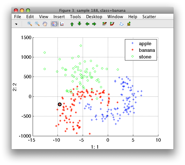
Lets make a fruit data set with second feature scaled by 100:

>> b=setdata(a, [+a(:,1) +a(:,2)*100])
'Fruit set' 260 by 2 sddata, 3 classes: 'apple'(100) 'banana'(100) 'stone'(60) 

>> sdscatter(b)

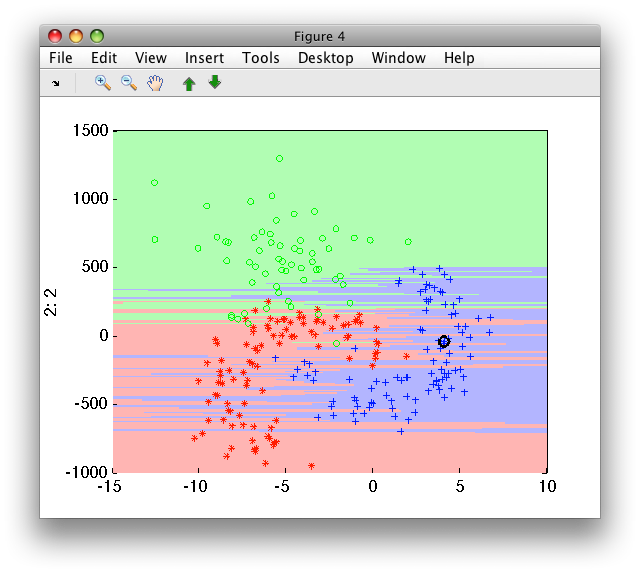
Scatter plot of a data set with strongly scaled feature.

If we train k-NN on this data, the classifier decisions will be strongly affected by incomparable scales of the two features:

>> pk1=sdknn(b)
sequential pipeline       2x1 '1-NN+Decision'
1 1-NN                    2x3  260 prototypes
2 Decision                3x1  weighting, 3 classes
>> sdscatter(b,pk1)

k-NN classifier result on data set with strongly scaled feature.

Training the k-NN on the scaled version makes both feature equally important. The sdscale by default yields zero mean and unit variance:

>> ps=sdscale(b)
Scaling pipeline          2x2  standardization
>> pk2=sdknn(b*ps)
sequential pipeline       2x1 '1-NN+Decision'
1 1-NN                    2x3  260 prototypes
2 Decision                3x1  weighting, 3 classes
>> sdscatter(b,ps*pk2)

k-NN classifier result on scaled data set.

Training of the k-NN on scaled data may be written on one line by constructing an untrained pipeline:

>> pu=sdscale*sdknn([],3)
untrained pipeline 2 steps: sdscale+sdknn

>> ptr=b*pu
sequential pipeline       2x1 'Scaling+3-NN+Decision'
1 Scaling                 2x2  standardization
2 3-NN                    2x3  260 prototypes
3 Decision                3x1  weighting, 3 classes

13.3.1.3. Different k-NN formulations ↩

By default, sdknn measures, for each class, a distance to the k-th nearest prototype. An alternative formulation finds k nearest prototypes irrespective of their classes and returns a fraction of each class among these k prototypes. The nearest neighbor computing class fractions is created by setting the method to classfrac:

>> p2=sdknn(a,10,'classfrac')
sequential pipeline       2x1 '10-NN discriminant+Decision'
 1 10-NN discriminant      2x3  260 prototypes
 2 Decision                3x1  weighting, 3 classes

Although both methods may look similar at the first sight, different way of computing the per-class output has important practical consequences. The distance method returns distance while the classfrac the similarity (fraction):

>> p1(1).output
ans =
distance

>> p2(1).output
ans =
posterior

Because classfrac is computing class fractions between k neighbors, it provides a discriminant applicable to two or more classes. This means that it splits the feature space into open sub-spaces. It separates classes but cannot be used to detect one class protecting it from all directions. The distance method, on the other hand, computes distance to k-th nearest neighbor for each class separately:

>> p=sdknn( a(:,:,'banana') ,10,'classfrac')
{??? Error using ==> sdknn at 209
k-NN with classfrac option cannot be used for one-class problems.
} 

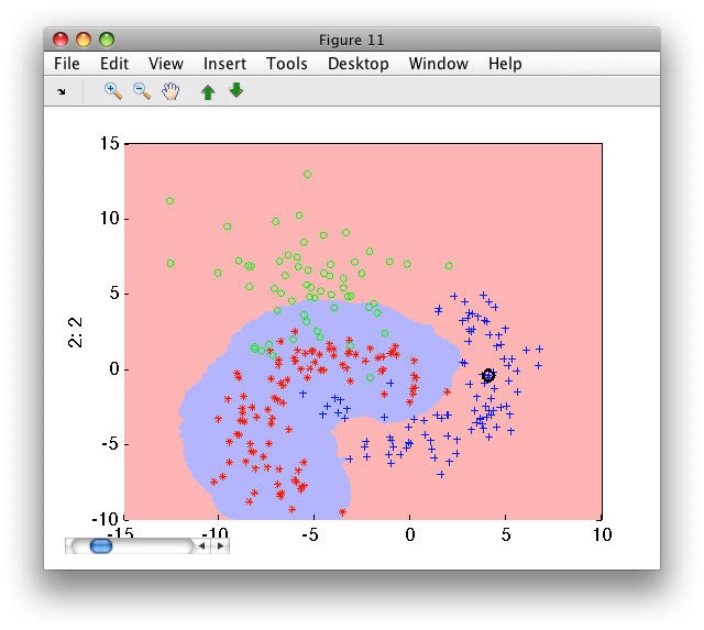
>> p=sdknn( a(:,:,'banana') ,10)
sequential pipeline       2x1 '10-NN+Decision'
1 10-NN                   2x1  100 prototypes
2 Decision                1x1  threshold on 'banana'
>> sdscatter(a,p)

Distance-based k-NN classifier as a one-class detector.

13.3.2. Prototype selection for k-NN ↩

By default sdknn uses all training examples as prototypes. It may, however, also select a smaller subset. Two prototype selection strategies are used:

random - selecting a specified number of prototypes per class
kcentres - using sdkcentres clustering algorithm to systematically select prototypes.

In this example, we randomly select 40 prototypes per class:

>> p=sdknn(a,'k',5,'proto',40)
sequential pipeline       2x1 '5-NN+Decision'
 1 5-NN                    2x3  120 prototypes
 2 Decision                3x1  weighting, 3 classes

Number of prototypes may be adjusted per class. Simpler classes may be described by smaller prototype sets. This increases execution speed of the k-NN classifier:

>> p=sdknn(a,'k',5,'proto',[40 40 10])
sequential pipeline       2x1 '5-NN+Decision'
 1 5-NN                    2x3  90 prototypes
 2 Decision                3x1  weighting, 3 classes

To select prototypes using kcentres, use protosel option:

>> p=sdknn(a,'k',5,'proto',40,'protosel','kcentres')
[class 'apple' 40 comp] 
[class 'banana' 40 comp] 
[class 'stone' 40 comp] 
sequential pipeline       2x1 '5-NN+Decision'
 1 5-NN                    2x3  120 prototypes
 2 Decision                3x1  weighting, 3 classes

k-centres algorithm computes dissimilarity matrix. For large data sets, sdknn uses only randomly drawn 2000 examples to compute k-centres.

13.3.3. k-means as a classifier ↩

k-means is a clustering approach where k cluster centers are derived by an iterative procedure minimizing mean (squared) distance of observation in each cluster.

perClass sdkmeans can be used for cluster analysis but is, by default, also a classifier. It performs the cluster optimization for each of the classes and outputs a 1-NN based-classifier. The prototypes of this classifier are the cluster centers.

The advantage of using k-means as a classifier is the systematic reduction of number of prototypes compared to a k-NN classifier that employes all training examples. This yields classifiers of comparable performance but significantly faster in execution.

>> load fruit_large
>> a
'Fruit set' 2000 by 2 sddata, 3 classes: 'apple'(667) 'banana'(667) 'stone'(666) 
>> p=sdkmeans(a,50)
[class 'apple' 13 iters.  9 clusters pruned,  41 clusters] 
[class 'banana' 19 iters.  14 clusters pruned,  36 clusters] 
[class 'stone' 18 iters.  10 clusters pruned,  40 clusters] 
sequential pipeline       2x1 '1-NN (k-means prototypes)+Decision'
 1 1-NN (k-means prototypes)    2x3  117 prototypes
 2 Decision                3x1  weighting, 3 classes

>> sdscatter(randsubset(a,200),p)

k-means used as a classifier.

By default, 200 iterations is performed unless a stable solution is reached. In the following example, we limit the number of iterations to 15. As we set identical random seed before running sdkmeans, we work exactly on the same data with identical initialization as above. Due to the iteration limit, we receive warning for the second and third classes:

>> rand('state',1); p=sdkmeans(a,50,'iter',15)
[class 'apple' 13 iters.  9 clusters pruned,  41 clusters] [class 'banana' 15 iters. {Warning: sdkmeans stopped without converging after the limit of 15 iterations.
Increase the max numbef of iterations using 'iter' option.}
 14 clusters pruned,  36 clusters] [class 'stone' 15 iters. {Warning: sdkmeans stopped without converging after the limit of 15 iterations.
Increase the max numbef of iterations using 'iter' option.} 
 10 clusters pruned,  40 clusters] 
sequential pipeline       2x1 '1-NN (k-means prototypes)+Decision'
 1 1-NN (k-means prototypes)    2x3  117 prototypes
 2 Decision                3x1  weighting, 3 classes

13.3.3.1. Adjusting number of centers in the k-means classifier ↩

Different k may be specified for each class. This is useful if we know that some classes are unimodal (like 'stone' on our example):

>> p=sdkmeans(a,[30 30 1])
[class 'apple' 6 clusters pruned,  24 clusters] [class 'banana' 10 clusters pruned,  20 clusters] [class 'stone' 1 clusters] 
sequential pipeline       2x1 '1-NN (k-means prototypes)+Decision'
1 1-NN (k-means prototypes)    2x3  45 prototypes
2 Decision                3x1  weighting, 3 classes

13.3.3.2. Changing k in the final k-NN classifier ↩

By default, sdkmeans returns a 1-NN classifier. This may be changed by the 'k final' option:

>> p=sdkmeans(a,50,'k final',2)
[class 'apple' 10 clusters pruned,  40 clusters] [class 'banana' 14 clusters pruned,  36 clusters] [class 'stone' 8 clusters pruned,  42 clusters] 
sequential pipeline       2x1 '2-NN (k-means proto)+Decision'
1 2-NN (k-means proto)    2x3  118 prototypes
2 Decision                3x1  weighting, 3 classes

An alternative is to change the k field in the resulting pipeline:

>> p(1).k=10
sequential pipeline       2x1 '10-NN+Decision'
1 10-NN                   2x3  118 prototypes
2 Decision                3x1  weighting, 3 classes

13.3.3.3. Prototype pruning ↩

By default, sdkmeans prunes prototypes in order to minimize misclassification in the areas of overlap. Pruning may be disabled with 'no pruning' option.

>> p=sdkmeans(a,50,'no pruning')
[class 'apple' 50 clusters] [class 'banana' 50 clusters] [class 'stone' 50 clusters] 
sequential pipeline       2x1 '1-NN (k-means prototypes)+Decision'
1 1-NN (k-means prototypes)    2x3  150 prototypes
2 Decision                3x1  weighting, 3 classes