
Classifiers, table of contents
This section describes support vector machines for classification.
- 13.7.1. Introduction
- 13.7.2. Linear support vector machine
- 13.7.3. Polynomial support vector machine
- 13.7.4. Grid search for sigma and C parameters
- 13.7.5. Multi-class using one-against-all approach
- 13.7.6. Multi-class using one-against-one approach
- 13.7.7. One-class support vector machines (RBF)
- 13.7.8. Repeatability of grid search
- 13.7.8.1. Fixing random seed
- 13.7.8.2. Split data outside
- 13.7.9. Probabilistic output for two-class SVM
13.7.1. Introduction ↩
perClass sdsvc command trains a support vector machine classifier using
libSVM library. The sdsvc supports linear, RBF and polynomial kernels.
The trained support vector machines are executed through the perClass
runtime library.
By default, RBF kernel is used with sigma and C parameters selected automatically based on a grid search. The mean error on a validation set (25% of the training set) is optimized during the grid search.
>> b
'Fruit set' 200 by 2 sddata, 2 classes: 'apple'(100) 'banana'(100)

>> p=sdsvc(b)
....................sigma=6.84618 C=234 err=0.000 SVs=24
sequential pipeline       2x1 'Scaling+Support vector machine+Decision'
 1 Scaling                 2x2  standardization
 2 Support vector machine    2x1  RBF kernel, sigma=6.85, 24 SVs
 3 Decision                1x1  threshold on 'apple'
sdsvc displays the sigma and C parameters together with the error on
validation set and number of support vectors. Keep in mind that the number
of support vectors is important indicator of well-trained support vector
machine. Large number of SVs may mean that we use wrong sigma or C or that
the libsvm optimizer did not find a good solution. The two-class support
vector machine yields one soft output which needs to be thresholded in
order to make a decision. This happens in the third step.
The number of support vectors used may be queried directly from the second step of the pipeline"
>> p(2)'
Support vector machine pipeline 2x1
 1 Support vector machine    2x1  RBF kernel, sigma=6.85, 24 SVs
       inlab: 'Feature 1','Feature 2'
         lab: 'apple'
      output: similarity
     svcount: support vector count

>> p(2).svcount

ans =

    24
Note that sdsvc performs scaling of input data by default. This may be
switched off using the 'noscale' option.
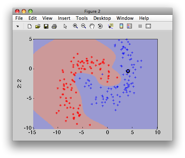
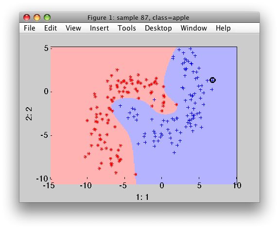
>> sdscatter(b,p)
13.7.2. Linear support vector machine ↩
Linear support vector machine is trained by specifying the kernel type 'linear':
>> p=sdsvc(b,'type','linear')
....................C=12.7 err=0.140 SVs=49
sequential pipeline       2x1 'Support vector machine+Decision'
 1 Support vector machine 2x1  linear
 2 Decision               1x1  threshold on 'apple'
By default, sdsvc performs search for the C parameter. The list of C
parameters may be also specified explicitly:
>> p=sdsvc(b,'type','linear','C',[1 2 5 10 100])
.....C=1 err=0.080 SVs=49
sequential pipeline       2x1 'Support vector machine+Decision'
 1 Support vector machine 2x1  linear
 2 Decision               1x1  threshold on 'apple'
Note that the explicit definition of 'type' is not required:
>> p=sdsvc(b,'linear','C',[1 2 5 10 100])
.....C=1 err=0.100 SVs=49
sequential pipeline       2x1 'Support vector machine+Decision'
 1 Support vector machine 2x1  linear
 2 Decision               1x1  threshold on 'apple'
13.7.3. Polynomial support vector machine ↩
Polynomial SVM optimizes degree and C parameters using a grid search.
>> p=sdsvc(b,'type','poly')
.....degree=4.00000 C=26.4 err=0.020 SVs=13
sequential pipeline       2x1 'Scaling+Support vector machine+Decision'
 1 Scaling                2x2  standardization
 2 Support vector machine 2x1  Polynomial kernel
 3 Decision               1x1  threshold on 'apple'
By default, the scaling is applied to the data (may be switched off using 'noscale' option).
Both degree and C parameters may be specified explicitly:
>> p=sdsvc(b,'type','poly','degree',[2 3 4 5],'C',[0.1 1 2 4 10 30 50 80])
....degree=3.00000 C=4 err=0.040 SVs=18
sequential pipeline       2x1 'Scaling+Support vector machine+Decision'
 1 Scaling                2x2  standardization
 2 Support vector machine 2x1  Polynomial kernel
 3 Decision               1x1  threshold on 'apple'
13.7.4. Grid search for sigma and C parameters ↩
sdsvc allows us to specify sigma and C parameters explicitly:
>> p=sdsvc(b,'sigma',1.5,'C',10)
SVs=21
sequential pipeline       2x1 'Scaling+Support vector machine+Decision'
 1 Scaling                2x2  standardization
 2 Support vector machine 2x1  RBF kernel, sigma=1.50, 21 SVs
 3 Decision               1x1  threshold on 'apple'
We may also specify the vector of sigmas and Cs. Second output of sdsvc
is a structure with estimated errors and numbers of support vectors:
>> [p,E]=sdsvc(b,'sigma',0.1:0.1:5,'C',[0.01 0.1 1 3 5 10 20])
..................................................sigma=1.30000 C=20 err=0.020 SVs=18
sequential pipeline       2x1 'Scaling+Support vector machine+Decision'
 1 Scaling                2x2  standardization
 2 Support vector machine 2x1  RBF kernel, sigma=1.30, 18 SVs
 3 Decision               1x1  threshold on 'apple'

E =

    sigmas: [1x50 double]
        Cs: [0.0100 0.1000 1 3 5 10 20]
       err: [50x7 double]
       svs: [50x7 double]
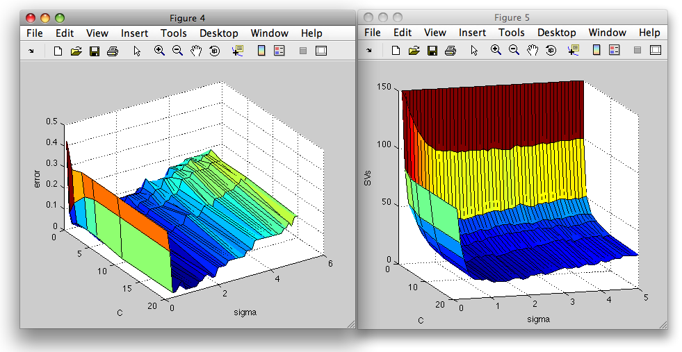
We may visualize the errors and number of suport vectors in a 3D surface plot:
>> figure; surf(E.Cs,E.sigmas,E.err)
>> xlabel('C'); ylabel('sigma'); zlabel('error')
>> figure; surf(E.Cs,E.sigmas,E.svs)
>> xlabel('C'); ylabel('sigma'); zlabel('SVs')
13.7.5. Multi-class using one-against-all approach ↩
By default, sdsvc uses one-against-all approach to train a multi-class
classifier. Separate grid-search is run for each of the sub-problems.
>> a
'Fruit set' 260 by 2 sddata, 3 classes: 'apple'(100) 'banana'(100) 'stone'(60)
>> p=sdsvc(a)
one-against-all: ['apple' ....................sigma=3.36900 C=2.98 err=0.037 SVs=47]
['banana' ....................sigma=0.48532 C=6.16 err=0.087 SVs=51]
['stone' ....................sigma=7.16612 C=12.7 err=0.010 SVs=31]
sequential pipeline 2x1 'Scaling+Support Vector Machine'
1 Scaling 2x2 standardization
2 stack 2x3 3 classifiers in 2D space
3 Decision 3x1 weighting, 3 classes
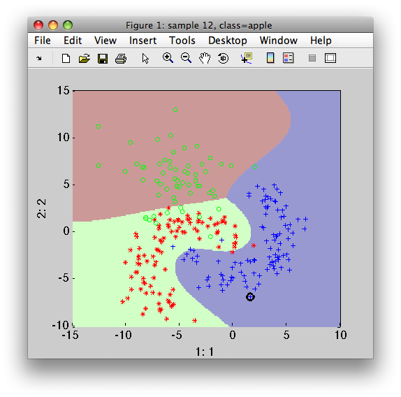
>> sdscatter(a,p)
Grid-search estimating errors in multi-class problems are returned in a cell
array with one E structure per class:
>> [p,E]=sdsvc(a,'sigma',0.1:0.1:5,'C',[0.01 0.1 1 3 5 10 20])
one-against-all: ['apple' ......................sigma=0.50000 C=5 err=0.025 SVs=38]
['banana' ......................sigma=0.20000 C=3 err=0.087 SVs=79]
['stone' ......................sigma=3.60000 C=5 err=0.000 SVs=32]
sequential pipeline       2x1 'Scaling+Support Vector Machine'
 1 Scaling                 2x2  standardization
 2 stack                   2x3  3 classifiers in 2D space
 3 Decision                3x1  weighting, 3 classes

>> E{2}

ans =

sigmas: [1x50 double]
    Cs: [0.0100 0.1000 1 3 5 10 20]
   err: [50x7 double]
   svs: [50x7 double]
13.7.6. Multi-class using one-against-one approach ↩
One-against-all approach often yields very complex individual classifiers as each class needs to be separated from all other classes. Therefore, large numbers of support vectors are typically needed. An alternative is the one-against-one approach. Here, we build pair-wise classifiers that are fundamentally simpler. On the other hand, for a C-class problem, C*(C-1)/2 classifiers are needed. While for three-class problem it is three classifiers, for four class problem it is six and for ten class problem 45 classifiers!
perClass sdsvc can adopt one-against-one strategy using identically-named option:
>> p=sdsvc(a,'one-against-one')
one-against-one: [1 of 3: 'apple' vs 'banana' ....................sigma=1.48911 C=483 err=0.000 SVs=11]
[2 of 3: 'apple' vs 'stone' ....................sigma=7.54766 C=2.98 err=0.033 SVs=17]
[3 of 3: 'banana' vs 'stone' ....................sigma=2.27747 C=234 err=0.000 SVs=21]
sequential pipeline       2x1 'Scaling+SVM stack+Multi-class combiner+Decision'
 1 Scaling                 2x2  standardization
 2 SVM stack               2x3  3 classifiers in 2D space
 3 Multi-class combiner    3x3
 4 Decision                3x1  weighting, 3 classes
Note that perClass implementation of one-against-one SVM still returns soft output (see the special combiner in step 3) instead of commonly-used crisp voting. Therefore, we may perform multi-class ROC optimization as with any other classifier.
13.7.7. One-class support vector machines (RBF) ↩
The RBF support verctor classifier may be trained on a single class. In such case, both sigma and C parameters must be provided:
>> a
'Fruit set' 260 by 2 sddata, 3 classes: 'apple'(100) 'banana'(100) 'stone'(60)

>> p=sdsvc( a(:,:,'banana'), 'sigma',0.3, 'C',1 )
sequential pipeline       2x1 'Scaling+Support vector machine+Decision'
 1 Scaling                 2x2  standardization
 2 Support vector machine    2x1  one-class RBF kernel, sigma=0.30, 64 SVs
 3 Decision                1x1  threshold on 'banana'

>> sdscatter(a,p)
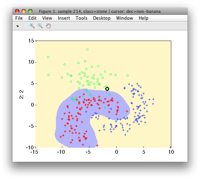
One-class SVM formulation may be used also in sddetect:
>> pd=sddetect(a,'banana',sdsvc([],'sigma',0.3,'C',1))
  1: apple  -> non-banana
  2: banana -> banana
  3: stone  -> non-banana
sequential pipeline       2x1 'Scaling+Support vector machine+Decision'
 1 Scaling                 2x2  standardization
 2 Support vector machine    2x1  one-class RBF kernel, sigma=0.30, 53 SVs
 3 Decision                1x1  ROC thresholding on banana (52 points, current 1)
13.7.8. Repeatability of grid search ↩
A grid search is performed when sdsvc meta-patameters such as sigma and C
for RBF kernel or degree and C for polynominal kernel are not specified.
Grid search splits the data internally, uses one part for training the
model and the other for evaluating model performance. This random data
splitting leads to slightly different results each time sdsvc is trained.
There are two possible solutions:
- fix random seed before the classifier training
- split data outside and provide both parts to
sdsvc
13.7.8.1. Fixing random seed ↩
Matlab random seed may be fixed before training sdsvc classifier.
Example:
>> rand('state',42); p1=sdsvc(b,'type','linear')
....................C=1.44 err=0.060 SVs=49
sequential pipeline       2x1 'Support vector machine+Decision'
 1 Support vector machine    2x1  linear
 2 Decision                1x1  threshold on 'apple'

>> rand('state',42); p2=sdsvc(b,'type','linear')
....................C=1.44 err=0.060 SVs=49
sequential pipeline       2x1 'Support vector machine+Decision'
 1 Support vector machine    2x1  linear
 2 Decision                1x1  threshold on 'apple'
Note identical outputs (C, error and number of support vectors).
13.7.8.2. Split data outside ↩
In order to have full control on classifier training perClass offers a consistent way how to deal with internal data splitting. We may split our data set outside the classifier and use the 'test' option to provide the part used for internal validation.
>> rand('state',1); [tr,ts]=randsubset(b,0.8)
'Fruit set' 160 by 2 sddata, 2 classes: 'apple'(80) 'banana'(80)
'Fruit set' 40 by 2 sddata, 2 classes: 'apple'(20) 'banana'(20)
Now, we provide the tr set as the first parameter and ts with the
'test' option:
>> p1=sdsvc(tr,'test',ts)
....................sigma=2.27784 C=113 err=0.025 SVs=12
sequential pipeline       2x1 'Scaling+Support vector machine+Decision'
 1 Scaling                 2x2  standardization
 2 Support vector machine    2x1  RBF kernel, sigma=2.28, 12 SVs
 3 Decision                1x1  threshold on 'apple'
Repeated training yields identical classifier:
>> p2=sdsvc(tr,'test',ts)
....................sigma=2.27784 C=113 err=0.025 SVs=12
sequential pipeline       2x1 'Scaling+Support vector machine+Decision'
 1 Scaling                 2x2  standardization
 2 Support vector machine    2x1  RBF kernel, sigma=2.28, 12 SVs
 3 Decision                1x1  threshold on 'apple'
To test it further, we may compare soft outputs of both pipelines (i.e. real-value output before conversion into a decision):
>> out1=ts*-p1
'Fruit set' 40 by 1 sddata, 2 classes: 'apple'(20) 'banana'(20)
>> out2=ts*-p2
'Fruit set' 40 by 1 sddata, 2 classes: 'apple'(20) 'banana'(20)
>> [+out1 +out2]

ans =

2.0170    2.0170
2.2087    2.2087
4.8025    4.8025
 ...