
This chapter describes construction and use of data sets.
- 5.1. Introduction
- 5.2. Constructing data sets
- 5.3. Importing and exporting data sets
- 5.3.1. Importing data sets
- 5.3.1.1. Importing multiple properties
- 5.3.2. Exporting data sets
- 5.4. Basic operations of data sets
- 5.4.1. Accessing samples, feature, and classes
- 5.4.2. Accessing raw data
- 5.4.3. Accessing class labels
- 5.5. Data set properties
- 5.5.1. Displaying available properties
- 5.5.2. Retrieving properties
- 5.5.3. Setting properties
- 5.5.3.1. Sample properties
- 5.5.3.2. Feature properties
- 5.5.3.3. Data properties
- 5.5.4. Testing presence of a property
- 5.5.5. Removing properties
- 5.6. Multiple sets of labels
- 5.7. Selecting data subsets by property values
- 5.8. Selecting data subsets randomly
- 5.9. Renaming classes and defining meta-classes
5.1. Introduction ↩
perClass stores data in sddata objects. sddata behaves
as a data matrix augmented with additional meta-data such as class labels
or feature names. The figure below provides a schematic illustration of
sddata object structure.
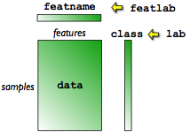
The data is stored in a matrix with rows corresponding to samples and
columns to features. Each data sample is thus represented by equal number
of features. A data sample belongs to a class. The class label is
accessible via the field called lab. The features names are stored in
the field featname.
5.2. Constructing data sets ↩
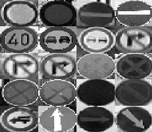
We will demonstrate the use of sddata object on a road sign example. We
will work with images of road sign boards (data samples), rescaled to a
common size of 32x32 pixels. Each road sign has a type such as "B2" or
"B28" which is a code from the transportation standard representing the
sign meaning such as "one-way" or "no-stopping". This picture shows 20
randomly selected road signs in our data base:
We will load the road sign data from the .mat file:
>> load data\road_signs.mat
>> whos
  Name             Size               Bytes  Class    Attributes

  data           381x1024            390144  uint8
  sign_type      381x4                 3048  char
The data matrix contains images of road sign boards, rescaled to 32x32
pixel raster and reshaped into 1x1024 vectors. For each sign, we also have
its type as string.
sddata object may be constructed by providing a matrix of numbers in
double precision.
>> a=sddata(double(data))
381 by 1024 sddata, class: 'unknown'
The object a is created which represents our data set. If we omit the
semicolon, Matlab displays size of the sddata object and some additional
information.
Note that all samples are labeled into the class 'unknown'. sddata set
always contains at least one class. If no class labels are provided, as in
our example, the default unknown class is assigned to all data samples.
We may provide the sample class labels in a character array directly when
constructing the sddata set:
>> a=sddata(double(data),sign_type)
381 by 1024 sddata, 17 classes: [31  28  24  33  19  21  57  26  21   9  13  15  14   1  14  29  26]
We can see that our data set now contains 17 classes. The standard display shows the per-class number of samples.
5.3. Importing and exporting data sets ↩
5.3.1. Importing data sets ↩
Data sets may be imported from comma-separated text file using the
sdimport command. Samples are assumed to be stored in rows and features
in columns.
>> data=rand(10,3)
% writing the numerical data in a text file:
>> dlmwrite('out.txt',data)
By default, sdimport assumes that the file contains only data
matrix. Here we load 10 samples each with 3 features.
>> b=sdimport('out.txt')
10 by 3 sddata, class: 'unknown'
Often, our data text file contains also labels. Lets assume the following file content:
0.28594,0.72406,0.82886,banana
0.39413,0.28163,0.16627,apple
0.50301,0.26182,0.39391,banana
0.72198,0.70847,0.52076,apple
0.30621,0.78386,0.71812,lemon
0.11216,0.98616,0.56919,lemon
0.44329,0.47334,0.46081,banana
0.46676,0.90282,0.44531,banana
0.014669,0.45106,0.087745,banana
0.66405,0.80452,0.44348,apple
We may load such data by specifying the column indices of the data matrix and of the labels:
>> b=sdimport('out.txt','data',1:3,'lab',4)
10 by 3 sddata, 3 classes: 'apple'(3) 'banana'(5) 'lemon'(2)
If the text file contains a header with comments, we may skip specific number of rows with the 'skip' option:
>> b=sdimport('out.txt','skip',2)
260 by 2 sddata, class: 'unknown'
The delimiter character may be changes using 'delimiter' option.
5.3.1.1. Importing multiple properties ↩
sdimport allows reading of multiple properties such as additional labels
or other sample meta-data. Let us consider the following file:
day 1,0.28594,0.72406,0.82886,banana
day 1,0.39413,0.28163,0.16627,apple
day 1,0.50301,0.26182,0.39391,banana
day 1,0.72198,0.70847,0.52076,apple
day 1,0.30621,0.78386,0.71812,lemon
day 2,0.11216,0.98616,0.56919,lemon
day 2,0.44329,0.47334,0.46081,banana
day 2,0.46676,0.90282,0.44531,banana
day 2,0.014669,0.45106,0.087745,banana
day 2,0.66405,0.80452,0.44348,apple
The first column specifies the day of data acquisition. We may use it as an additional label to understand differences between class distributions at different days.
We may load multiple sample properties using the 'columns' option. It takes
a cell array argument with property name and column indices. We may also
specify data type for the additional properties, such as 'day' in our
example. By default, the properties are assumed to be numerical. For
sdlab labels, use L: name prefix, for strings S: and for cell
arrays C:. Here, we read 'day' as a label:
>> b=sdimport('out.txt','columns',{'data',2:4,'lab',5,'L:day',1})
10 by 3 sddata, 3 classes: 'apple'(3) 'banana'(5) 'lemon'(2)
>> b.day
sdlab with 10 entries, 2 groups: 'day 1'(5) 'day 2'(5)
>> +b.day

ans =

day 1
day 1
day 1
day 1
day 1
day 2
day 2
day 2
day 2
day 2
5.3.2. Exporting data sets ↩
Data sets may be exported to a comma-separated file using the sdexport
command. Currently, sdexport outputs only data matrix and labels.
>> a
'Fruit set' 260 by 2 sddata, 3 classes: 'apple'(100) 'banana'(100) 'stone'(60)

>> sdexport(a,'out.txt')
File 'out.txt' contains:
% data (2 features), lab
% import using: a=sdimport('out.txt','skip',2,'data',1:2,'lab',3)
4.02448560336199,-0.42381726996063,apple
1.00152794339117,-4.72599270607262,apple
3.22400075820392,2.62942331818164,apple
3.78787304139792,-3.94519946922846,apple
2.36436674935594,-5.60064442112387,apple
...
Note that the file contains a header listing the content (data matrix with
2 features and labels). Second line contains the sdimport command that
may be used for quick reading of this text file into perClass.
5.4. Basic operations of data sets ↩
5.4.1. Accessing samples, feature, and classes ↩
sddata behaves as a matrix with rows representing data samples and
columns representing features.
To extract first 40 samples from the data set, use:
>> b=a(1:40)
40 by 1024 sddata, 4 classes: 'C3'(9) 'C4b'(13) 'C4c'(15) 'C4d'(3)
Note that the resulting data set b contains only four classes. Empty
classes are automatically removed. For small numbers of classes, sddata
display provides also the class names and sample counts.
To extract a subset of features, we provide column indices:
>> c=a(:,1:10)
381 by 10 sddata, 17 classes: [31  28  24  33  19  21  57  26  21   9  13  15  14   1  14  29  26]
Besides sample and feature subsets, we often need to access all samples
assigned to a specific class. perClass makes the handling of classes
very easy. In addition to samples and features, the third "dimension" of
any sddata object refers to the class:
>> size(a)
ans =
     381        1024          17
Frequently used task is to find the number of classes:
>> size(a,3)
ans =
      17
The number of samples may be directly obtained using the length function:
>> length(a)
ans =
   381
Note, that the length operator always returns number of samples (and not, the largest dimension as is Matlab convention for matrices).
To return samples of a specific class, we may simply provide its name as the third argument:
>> a(:,:,'C3')
9 by 1024 sddata, class: 'C3'
Subset of classes may be retrieved by providing a cell array with class names:
>> a(:,:,{'C3','B1'})
40 by 1024 sddata, 2 classes: 'B1'(31) 'C3'(9)
5.4.2. Accessing raw data ↩
Data values may be accessed using the double or unary plus operator:
>> +a(1:3,1:2)
ans =
   207   207
62    59
85   110

>> double(a(1:3,1:2))
ans =
   207   207
    62    59
    85   110
To quickly access raw data for a specific class, say 'B2', use:
>> data=+a(:,:,'B2');

>> size(data)
ans =
      28        1024
To compute mean or covariance matrix per class, use mean and
cov methods. mean returns sddata object with
mean per class. cov returns a cell array with covariance matrix
per class:
>> m=mean(a(:,:,1:4))
4 by 1024 sddata, 4 classes: 'B1'(1) 'B2'(1) 'B20a'(1) 'B21a'(1)

>> cov(a(:,:,1:4))
ans =
  Columns 1 through 3
[1024x1024 double]    [1024x1024 double]    [1024x1024 double]
  Column 4
[1024x1024 double]
5.4.3. Accessing class labels ↩
Class labels may be retrieved using getlab method:
>> getlab(a)
sdlab with 381 entries, 17 groups
The labels are stored in a sdlab object discussed in detail here. To access the string names, use the unary plus
operator:
>> lab=getlab(a(1:12))
sdlab with 12 entries, 2 groups: 'C3'(9) 'C4b'(3)

>> +lab
ans =
C3
C3
C3
C3
C3
C3
C3
C3
C3
C4b
C4b
C4b
Each sdlab object contains a list of class names:
>> a.lab.list
sdlist (2 entries)
 ind name
   1 C3
   2 C4b
Displaying the list allows us to see the order of classes.
5.5. Data set properties ↩
perClass introduces the concept of properties. Property is any
user-accessible part of the sddata object. sddata uses the structure
metaphor and exposes its data properties as fields. For example, the raw
data content of the sddata object a is accessible using a.data and
sample labels using a.lab.
There are three types of properties, referring to samples, features and to
the entire data set. For example, class label is a property of a data
sample and feature name of a data set feature (column). Data properties
refer to the complete data set. We may, for example, add a timestamp
property defining acquisition time.
All sddata objects share some default properties such as data (data
matrix), lab (sample class labels) or featlab (feature labels or
names). These properties cannot be removed.
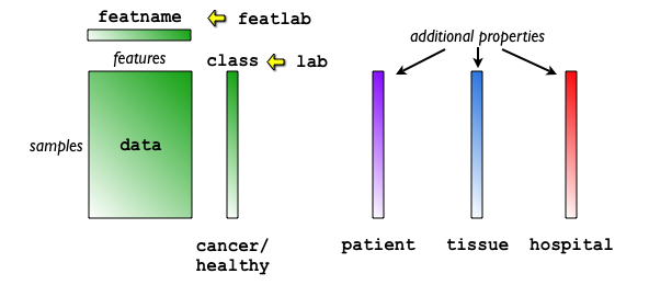
User may add any number of custom properties describing problem specific meta-data. For example, when working with medical data, we may wish to attach patient id to each data sample. This allows us to visualize class distribution in each patient.
In the schema below few properties are added to the data, beside the
primary label cancer\healthy. It is the patient id, the tissue type and
the hospital that generated the data set. Multiple labels is a powerful
tool that allows a better understanding of the problem at hand. The labels
may be inspected with the interactive visualization tools, but also used
for a robust classifier evaluation. See the example of cross-validation over properties.
5.5.1. Displaying available properties ↩
Simple way to display the list of properties is to use the transpose operator:
>> a'
381 by 1024 sddata, 17 classes: [31  28  24  33  19  21  57  26  21   9  13  15  14   1  14  29  26]
sample props: 'lab'->'class' 'class'(L)
feature props: 'featlab'->'featname' 'featname'(L)
data props:  'data'(N)
We can see separately the sample, feature and data properties. Note the special 'lab' and 'featlab' properties that act as a proxy pointing to the current sample labels (by default 'class') and feature labels (by default 'featname'), respectively. Details about switching between multiple labels is described in the next section.
Second way to access names of available properties is using the
getproplist method:
>> getproplist(a)
ans =
'class'
By default, it presents us with the list (cell array) of sample properties. To list the feature or data properties, use an additional argument:
>> getproplist(a,'feat')
ans =
'featname'

>> getproplist(a,'data')
ans =
'data'
5.5.2. Retrieving properties ↩
To access content of a property, simply use the familiar Matlab dot notation for structure fields:
>> a.class
sdlab with 381 entries, 17 groups
This is analogous to calling the getprop method:
>> getprop(a,'class')
sdlab with 381 entries, 17 groups
We may retrieve property of any type using getprop or field access.
5.5.3. Setting properties ↩
5.5.3.1. Sample properties ↩
To set a property we may use the field assignment. For example, we may create a new sample label defining on which day was a road sign image (sample) acquired.
>> video=sdlab('day 1',200,'day 2',100,'day 3',81)
sdlab with 381 entries, 3 groups: 'day 1'(200) 'day 2'(100) 'day 3'(81)

>> a.video=video
381 by 1024 sddata, 17 classes: [31  28  24  33  19  21  57  26  21   9  13  15  14   1  14  29  26]

>> a'
381 by 1024 sddata, 17 classes: [31  28  24  33  19  21  57  26  21   9  13  15  14   1  14  29  26]
sample props: 'lab'->'class' 'class'(L) 'video'(L)
feature props: 'featlab'->'featname' 'featname'(L)
data props:  'data'(N)
Alternative approach is based on the setprop method:
>> a=setprop(a,'video',video)
381 by 1024 sddata, 17 classes: [31  28  24  33  19  21  57  26  21   9  13  15  14   1  14  29  26]
Property may be also any matrix or cell array. The only requirement is that its first dimension is equal to the number of samples.
We may, for example, create a sample property 'id' holding a unique number for each sample.
>> a.id=1:length(a)
381 by 1024 sddata, 17 classes: [31  28  24  33  19  21  57  26  21   9  13  15  14   1  14  29  26]

>> a'
381 by 1024 sddata, 17 classes: [31  28  24  33  19  21  57  26  21   9  13  15  14   1  14  29  26]
sample props: 'lab'->'class' 'class'(L) 'video'(L) 'id'(N)
feature props: 'featlab'->'featname' 'featname'(L)
data props:  'data'(N)
The 'id' property may help us to identify a specific sample in a data subset.
Properties may be assigned directly:
>> a(1:5).lab='newsign';
Or
>> a.lab(1:5)='newsign'
381 by 1024 sddata, 18 classes: [31  28  24  33  19  21  57  26  21   4  13  15  14   1  14  29  26   5]
>> a.lab'
 ind name       size percentage
   1 B1           31 ( 8.1%)
   2 B2           28 ( 7.3%)
   3 B20a         24 ( 6.3%)
   4 B21a         33 ( 8.7%)
   5 B24a         19 ( 5.0%)
   6 B24b         21 ( 5.5%)
   7 B28          57 (15.0%)
   8 B29          26 ( 6.8%)
   9 B4           21 ( 5.5%)
  10 C3            4 ( 1.0%)
  11 C4b          13 ( 3.4%)
  12 C4c          15 ( 3.9%)
  13 C4d          14 ( 3.7%)
  14 C4e           1 ( 0.3%)
  15 C4f          14 ( 3.7%)
  16 C5a          29 ( 7.6%)
  17 C5b          26 ( 6.8%)
  18 newsign       5 ( 1.3%)
5.5.3.2. Feature properties ↩
Given an additional 'feat' argument, setprop sets a feature property.
Setting a feature property may be useful when subsets of out features are computed with different feature extractor software (or version) and we wish to preserve knowledge of this grouping. Multiple feature labels are also present when computing similarity-based data representation.
>> b=a(:,1:10) %  lets use 10 features in this example

>> featgroup=sdlab('Group 1',4,'Group 2',6)
sdlab with 10 entries, 2 groups: 'Group 1'(4) 'Group 2'(6)

>> b=setprop(b,'featgroup',featgroup,'feat')
381 by 10 sddata, 17 classes: [31  28  24  33  19  21  57  26  21   9  13  15  14   1  14  29  26]

>> b'
381 by 10 sddata, 17 classes: [31  28  24  33  19  21  57  26  21   9  13  15  14   1  14  29  26]
sample props: 'lab(class)' 'class' 'video' 'id'
feature props: 'featlab(featname)' 'featname' 'featgroup'
data props:  'data' 'date'

>> b.featgroup
sdlab with 10 entries, 2 groups: 'Group 1'(4) 'Group 2'(6)
Feature property may be any sdlab object, matrix, character array or cell array with the first dimension equal to the number of features.
5.5.3.3. Data properties ↩
Data properties are set using setprop with additional 'data'
argument.
Useful custom data property may be, for example, the timestamp of data set creation:
>> str=datestr(now)

str =

22-Jul-2013 15:04:51

>> a=setprop(a,'timestamp',str,'data')
381 by 1024 sddata, 17 classes: [31  28  24  33  19  21  57  26  21   9  13  15  14   1  14  29  26]
>> a'
381 by 1024 sddata, 17 classes: [31  28  24  33  19  21  57  26  21   9  13  15  14   1  14  29  26]
sample props: 'lab'->'class' 'class'(L)
feature props: 'featlab'->'featname' 'featname'(L)
data props:  'data'(N) 'timestamp'(S)
>> a.timestamp

ans =

22-Jul-2013 15:04:51
There is no constrain on type or format of data properties.
5.5.4. Testing presence of a property ↩
To check if a property exists, use isprop method. It takes data set and
property name and returns logical value:
>> a'
381 by 1024 sddata, 17 classes: [31  28  24  33  19  21  57  26  21   9  13  15  14   1  14  29  26]
sample props: 'lab'->'class' 'class'(L) 'video'(L) 'id'(N)
feature props: 'featlab'->'featname' 'featname'(L)
data props:  'data'(N)

>> isprop(a,'video')
ans =
 1

>> isprop(a,'frame')
ans =
 0
As the second output argument, isprop returns the property type
('sample','feat' or 'data'). For non existent properties, empty matrix []
is returned.
>> [i,t]=isprop(a,'video')
i =
 1
t =
sample

>> [i,t]=isprop(a,'other_property')
i =
 0
t =
 []
5.5.5. Removing properties ↩
Properties may be removed using rmprop method.
>> a'
381 by 1024 sddata, 17 classes: [31  28  24  33  19  21  57  26  21   9  13  15  14   1  14  29  26]
sample props: 'lab(class)' 'class' 'video' 'id'
feature props: 'featlab(featname)' 'featname'
data props:  'data' 'date'

>> a2=rmprop(a,'video')
381 by 1024 sddata, 17 classes: [31  28  24  33  19  21  57  26  21   9  13  15  14   1  14  29  26]

>> a2'
381 by 1024 sddata, 17 classes: [31  28  24  33  19  21  57  26  21   9  13  15  14   1  14  29  26]
sample props: 'lab(class)' 'class' 'id'
feature props: 'featlab(featname)' 'featname'
data props:  'data' 'date'
The properties used for 'lab' and 'featlab' proxies and 'data' property cannot be removed.
Alternatively, we may remove a property by assigning empty value []:
>> a2.id=[];
>> a2'
381 by 1024 sddata, 17 classes: [31  28  24  33  19  21  57  26  21   9  13  15  14   1  14  29  26]
sample props: 'lab(class)' 'class'
feature props: 'featlab(featname)' 'featname'
data props:  'data' 'date'
5.6. Multiple sets of labels ↩
Many pattern recognition problems benefit from using more than one set of
labels. For example, in road sign recognition we may investigate separately
class distribution inside urban areas or along the highways. sddata
object makes it easy to work with multiple sets of labels. Any indexed
property (an instance of sdlab class) may be used as a label set.
sddata introduces a simple mechanism allowing the user to choose which
property is currently considered as labels. This mechanism uses a special
property called 'lab' which points to an indexed property used as
labels. By default, 'lab' points to 'class'. We may access the 'lab'
property directly or using getlab as explained above:
>> a.lab
sdlab with 381 entries, 17 groups

>> getlab(a)
sdlab with 381 entries, 17 groups
By default, the getlab command is just proxied into the getprop call such as:
>> getprop(a,'class')
sdlab with 381 entries, 17 groups
In order to use a different set of labels, use setlab method. In the section above, we have added a new 'video' property
representing the day of video acquisition:
>> b.video
sdlab with 381 entries, 3 groups: 'day 1'(200) 'day 2'(100) 'day 3'(81)
We may now switch labels to video using:
>> b=setlab(a,'video')
381 by 1024 sddata, 3 'video' groups: 'day 1'(200) 'day 2'(100) 'day 3'(81)

>> getlab(b)
sdlab with 381 entries, 3 groups: 'day 1'(200) 'day 2'(100) 'day 3'(81)

>> b.lab
sdlab with 381 entries, 3 groups: 'day 1'(200) 'day 2'(100) 'day 3'(81)
To display more details on available properties, use the transpose operator:
>> a'
381 by 1024 sddata, 17 classes: [31  28  24  33  19  21  57  26  21   9  13  15  14   1  14  29  26]
sample props: 'lab(class)' 'class' 'video' 'id'
feature props: 'featlab(featname)' 'featname'
data props:  'data' 'date'

>> b'
381 by 1024 sddata, 3 'video' groups: 'day 1'(200) 'day 2'(100) 'day 3'(81)
sample props: 'lab(video)' 'class' 'video' 'id'
feature props: 'featlab(featname)' 'featname'
data props:  'data' 'date'
Only indexed properties (instances of sdlab) may be used as
labels. Attempting to set other property types as labels results in error:
>> b=setlab(a,'id')
??? Error using ==> sddata.setlab at 53
Only indexed properties (sdlab) may be used as labels
To find out the name of the property used by 'lab', use the setlab method
without further arguments:
>> setlab(a)
ans =
class

>> setlab(b)
ans =
video
TIP: When writing your custom algorithms, access labels through the lab
proxy. In this way, the function will be directly applicable to any
user-defined set of labels.
5.7. Selecting data subsets by property values ↩
Subsets of data defined by property values may be retrieved using subset
method. In the simplest form, it takes the data set object and label value:
>> subset(a,'C3')
9 by 1024 sddata, class: 'C3'

>> subset(a,{'C3','C4b'})
22 by 1024 sddata, 2 classes: 'C3'(9) 'C4b'(13)
Alternatively to a name, we may specify classes using regular expression. Regular expression startts with the slash character (/). Classes matching the pattern are returned:
>> subset(a,'/B24')
40 by 1024 sddata, 2 classes: 'B24a'(19) 'B24b'(21)
The substring B24 matches two class names, B24a and B24b.
To query arbitrary properties, use the extended subset form specifying
the property name and value:
>> subset(b,'video','day 2')
100 by 1024 sddata, 'video' lab: 'day 2'
Multiple subset queries may be combined. We may be interested, for example,
in all B28 signs ("no stopping") acquired on day 2:
>> subset(b,'video','day 2','class','B28')
2 by 1024 sddata, 'video' lab: 'day 2'
The second output of subset provides the rest of the data set:
>> [c,d]=subset(a2,'B2')
28 by 1024 sddata, class: 'B2'
88 by 1024 sddata, 3 classes: 'B1'(31) 'B20a'(24) 'B21a'(33)
Third and fourth arguments return indices for the subset and remainder, respectively:
>> [c,d,ind1,ind2]=subset(a2,'B2');

>> c=a2(ind1)
28 by 1024 sddata, class: 'B2'

>> d=a2(ind2)
88 by 1024 sddata, 3 classes: 'B1'(31) 'B20a'(24) 'B21a'(33)
Low-level querying by property values is implemented by the sddata find
method. It has the same syntax as subset, only returns the sample
indices:
>> find(b,'video','day 2','class','B28')
ans =
   299
   300
The find query can also be used with regular expressions. The example below shows how to retrieve the indices of the classes that contais B24 or C5.
>> ind=find(a, '/ B24|C5');
>> length(ind)
ans =
    55
5.8. Selecting data subsets randomly ↩
Random subsets of an sddata set may be selected using randsubset
method. It operates on per-class basis using the current lab
setting. This means that the call
>> randsubset(b,10)
30 by 1024 sddata, 3 'video' groups: 'day 1'(10) 'day 2'(10) 'day 3'(10)
returns 10 objects per class. Instead of number of objects per class, we may specify the fraction:
>> randsubset(b,0.2)
76 by 1024 sddata, 3 'video' groups: 'day 1'(40) 'day 2'(20) 'day 3'(16)
If a different number of samples is desirable in each class, we may provide a vector of sample sizes:
>> randsubset(b,[5 10 20])
35 by 1024 sddata, 3 'video' groups: 'day 1'(5) 'day 2'(10) 'day 3'(20)
To select a subset of samples from the complete data set irrespective of
classes, we provide an additional all parameter:
>> randsubset(b,10,'all')
10 by 1024 sddata, 3 'video' groups: 'day 1'(6) 'day 2'(3) 'day 3'(1)

>> randsubset(b,10,'all')
10 by 1024 sddata, 2 'video' groups: 'day 1'(5) 'day 3'(5)
Note that some classes may disappear not being selected.
5.8.1. Splitting data for training and testing ↩
Often used idiom is a data split into training and test sets. randsubset
makes this simple by returning the remainder of the data set in the second
output argument:
>> a
381 by 1024 sddata, 17 classes: [31  28  24  33  19  21  57  26  21   9  13  15  14   1  14  29  26]

>> a2=a(:,:,1:4)
116 by 1024 sddata, 4 classes: 'B1'(31) 'B2'(28) 'B20a'(24) 'B21a'(33)

>> [tr,ts]=randsubset(a2,10)
40 by 1024 sddata, 4 classes: 'B1'(10) 'B2'(10) 'B20a'(10) 'B21a'(10)
76 by 1024 sddata, 4 classes: 'B1'(21) 'B2'(18) 'B20a'(14) 'B21a'(23)
5.8.2. Fixing the random state ↩
randsubset leverages Matlab random number generator. We should,
therefore, set the random state before calling it to get repeatedly
identical sample subset:
>> rand('state',42) %  fixing random state
>> c=randsubset(b,10,'all')
10 by 1024 sddata, 3 'video' groups: 'day 1'(6) 'day 2'(2) 'day 3'(2)
>> +c(1,1:3)
ans =
49    47    43

>> rand('state',42)
>> c=randsubset(b,10,'all') %  the same subset
10 by 1024 sddata, 3 'video' groups: 'day 1'(6) 'day 2'(2) 'day 3'(2)
>> +c(1,1:3)
ans =
49    47    43

>> c=randsubset(b,10,'all') %  now we get a different subset
10 by 1024 sddata, 3 'video' groups: 'day 1'(7) 'day 2'(2) 'day 3'(1)
>> +c(1,1:3)
ans =
86    85    87
5.9. Renaming classes and defining meta-classes ↩
It is often useful to define new classification problems by renaming the existing classes. For example, in the road sign problem, we might be interested building classifiers for the high-level groups of prohibitive signs (with red/white/black boards), red/blue no-stopping/parking signs and blue/white obligatory signs.
perClass provides the sdrelab command that allows us to quickly
relabel the sddata set or sdlab. sdrelab takes a data set and a cell
array with class re-writing rules of the format:
{ existing_class new_class ...}
The existing class may be specified by name or index. When using indices, we can easily refer to a group of existing classes in the input data. In the road sign example:
>> a
381 by 1024 sddata, 17 classes: [31  28  24  33  19  21  57  26  21   9  13  15  14   1  14  29  26]
>> c=sdrelab(a,{[1:6 9] 'prohibitive' 7:8 'nostop' 10:17 'obligatory'})
  1: B1     -> prohibitive
  2: B2     -> prohibitive
  3: B20a   -> prohibitive
  4: B21a   -> prohibitive
  5: B24a   -> prohibitive
  6: B24b   -> prohibitive
  7: B28    -> nostop
  8: B29    -> nostop
  9: B4     -> prohibitive
 10: C3     -> obligatory
 11: C4b    -> obligatory
 12: C4c    -> obligatory
 13: C4d    -> obligatory
 14: C4e    -> obligatory
 15: C4f    -> obligatory
 16: C5a    -> obligatory
 17: C5b    -> obligatory
381 by 1024 sddata, 3 classes: 'prohibitive'(177) 'nostop'(83) 'obligatory'(121)
The same task is simpler with regular expressions, where we specify the substrings instead of class indices:
>> d=sdrelab(a,{'/B28|B29','nonstop','/B','prohibitive','/C','obligatory'})
  1: B1     -> prohibitive
  2: B2     -> prohibitive
  3: B20a   -> prohibitive
  4: B21a   -> prohibitive
  5: B24a   -> prohibitive
  6: B24b   -> prohibitive
  7: B28    -> nonstop
  8: B29    -> nonstop
  9: B4     -> prohibitive
 10: C3     -> obligatory
 11: C4b    -> obligatory
 12: C4c    -> obligatory
 13: C4d    -> obligatory
 14: C4e    -> obligatory
 15: C4f    -> obligatory
 16: C5a    -> obligatory
 17: C5b    -> obligatory
381 by 1024 sddata, 3 classes: 'nonstop'(83) 'prohibitive'(177) 'obligatory'(121)
First, we labeled classes matching B28 OR B29 into nostop, then all
the classes containing B will became prohibitive and, finally, the ones
containing C were labeled obligatory.
sdrelab also allows us to define the existing classes by the negation
operator ~ (tilde). In this way, we can quickly relabel all classes other
than a specific class. Here, we will relabel the signs, that are not
prohibitive, as others:
>> d=sdrelab(c,{'~prohibitive','others'})
  1: prohibitive -> prohibitive
  2: nostop -> others
  3: obligatory -> others
381 by 1024 sddata, 2 classes: 'prohibitive'(177) 'others'(204)
To suppress printing of the conversion table, use 'nodisplay' option:
>> d=sdrelab(c,{'~prohibitive','others'},'nodisplay')
381 by 1024 sddata, 2 classes: 'prohibitive'(177) 'others'(204)
To rename all classes into one use the 'all' option:
>> d=sdrelab(a,'all','road signs')
381 by 1024 sddata, class: 'road signs'
5.9.1. Adding prefix or suffix to all class names ↩
sdrelab allows us to add a prefix or suffix string to all class names with
one command. This is useful, for example, when comparing two versions of
the same data set when analyzing effects of updated feature computation or
sensor normalization.
We may add the prefix 'old' to the classes in old data set, concatenate the
old and new data sets and visualize the total set using sdscatter. This
will allow us to visually separate old and new object instances.
>> load fruit
260 by 2 sddata, 3 classes: 'apple'(100) 'banana'(100) 'stone'(60)

>> a_old=sdrelab(a,'add','old-')
260 by 2 sddata, 3 classes: 'old-apple'(100) 'old-banana'(100) 'old-stone'(60)
The option 'add' is a synonym for 'prefix'. sdrelab also provides the
'suffix' option.