
- 7.1. Introduction
- 7.2. Visualizing images with sdimage
- 7.3. Creating image data sets objects directly
- 7.4. Hand-painting class labels
- 7.5. Cropping images
- 7.6. Saving image data set to workspace
- 7.7. Working with image subsets
- 7.8. Creating image matrix from a data set
- 7.9. Storing multiple images in data sets
- 7.10. Connecting sdimage and sdscatter
- 7.11. Clustering image with k-means
- 7.12. Defining connected components
7.1. Introduction ↩
perClass provides a set of tools for working with image data. It allows us
to visualize gray-level or multi-band images, compute local image features
and identify connected components. Starting with perClass 4, this
functionality is available as "Imaging option" (see sdversion for
available options).
7.2. Visualizing images with sdimage ↩
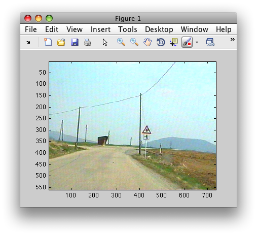
Let us consider an RGB image of a traffic scene 'roadsign09.bmp', loaded
with Matlab imread command:
>> im = imread('roadsign09.bmp');
>> figure; imagesc(im)
Using sdimage command on matrix im opens an interactive viewer:
>> sdimage(im);
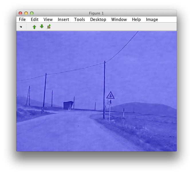
The blue layer on top of the image represents the set of labels of the
image data set, internally used by sdimage. As any other sddata
set, each sample (pixel) has a label, which is set to "unknown" by default.
We may toggle this label layer using the space bar key. Additionally, we
may also adjust label transparency from very transparent to opaque in the
Image menu.
The three image channels are visualized as three separate image bands. We
can move between the bands with the 'up' and 'down' cursor keys or the green arrows icons in the menu'. Each pixel is a data sample, the figure title shows the pixel's value and class label
('unknown' by default). sdimage loads the image if provided with the string filename:
>> sdimage('roadsign09.bmp')
7.3. Creating image data sets objects directly ↩
sdimage command allows us to create image data set directly on the Matlab
prompt using 'sddata' option:
>> a=sdimage(im,'sddata')
412160 by 3 sddata, class: 'unknown'
sdimage also accepts the image filename, attempting to load the file
using imread:
>> b=sdimage('roadsign11.bmp','sddata')
412160 by 3 sddata, class: 'unknown'
The objects a and b are standard sddata sets with one sample
for each pixel and three features corresponding to R,G, and B bands
respectively. Note, that the pixel values were also converted into double
precision.
7.4. Hand-painting class labels ↩
The interactive sdimage figure allows us to paint class labels for image
regions. In order to enter the 'paint' mode, use the Paint menu in the
Image menu, select the Create new class command:
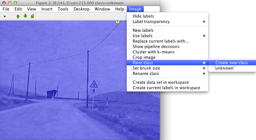
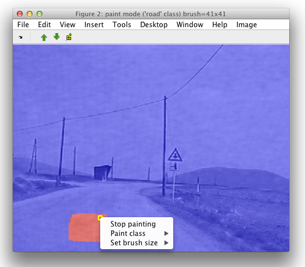
A dialog window will ask for the name of the class. Let's say we are interested in labeling the road, we provide the name of the class and paint in the image region. Via the Image menu, or by clicking the right mouse button we can change brush size or exit from the paint mode.
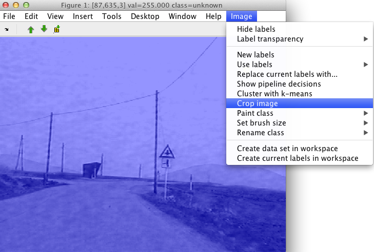
7.5. Cropping images ↩
Often, we only want to work with a smaller area of a large image.
sdimage offers us a crop function which makes this very quick.
Select the Crop image item in the Image menu.
A cross-hair will appear. Choose two corners of a region you wish to crop. The process may be terminated by clicking right mouse button.
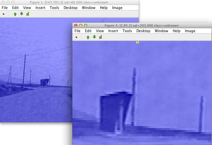
The new sdimage figure is opened containing the data from the specified
region. Cropped data contains all labels and properties of the complete
image. The image size for the new data set will be set to the specified
region. If you save the cropped image into data set c:
>> Creating data set c in the workspace.
12840 by 3 sddata, class: 'unknown'
>> getiminfo(a)

ans =

imsize: [560 736]

>> getiminfo(c)

ans =

imsize: [105 202]
7.6. Saving image data set to workspace ↩
The Create data set in workspace command in Image menu lets us to store
the image data together with the painted labels in a new sddata
object in the Matlab workspace. We are asked to provide the variable name for
this new data set.
Storing our image data set with the labeled road region in data2
variable, we will see the following message in Matlab command window:
>> Creating data set data2 in the workspace.
412160 by 3 sddata, 2 classes: 'unknown'(402557) 'road'(9603)
Alternatively, we may access the data set in any open open image figure with 'getdata' option, providing the figure handle:
>> sdimage(12,'getdata')
412160 by 3 sddata, 2 classes: 'unknown'(402454) 'road'(9706)
7.7. Working with image subsets ↩
The image data sets preserve the image information. We may, for example, use
only a subset of data, e.g. the pixels labeled as 'road' in the data2
object above.
>> sub=data2(:,:,'road')
9603 by 3 sddata, class: 'road'
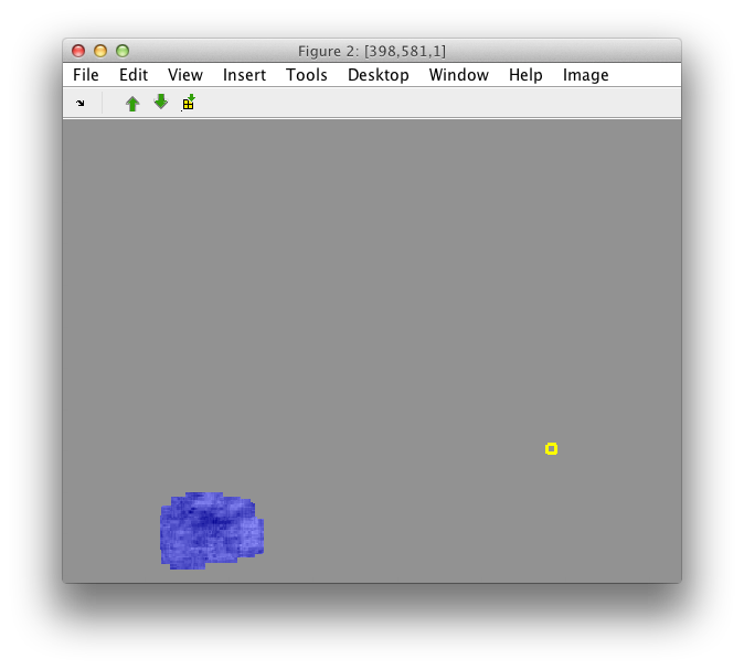
The image subset may be still visualized as an image:
>> sdimage(sub)
7.8. Creating image matrix from a data set ↩
The data set representation of image data is useful for training pattern
recognition algorithms. However, often we may need to apply imaging
operations, such as filtering, to our image regions. sdimage allows us to
create an image matrix with pixel values using the matrix option:
>> sub
9159 by 3 sddata, class: 'road'

>> I=sdimage(sub,'matrix');

>> size(I)

ans =

   560   736     3
Matrix I is created with the size of the original image the sub data
was extracted from. The matrix is filled with zeros and only the pixels
available in the sub data set are inserted into this matrix.
Note that the matrix I uses double precision:
>> class(I)

ans =

double
We may now perform any image processing operation such as filtering, and bring
the resulting data back into a data set format. This can be done using the
linear indices stored in the sub data set 'pixel' property:
>> sub2=setdata(sub, I(sub.pixel))
9159 by 1 sddata, class: 'road'
7.9. Storing multiple images in data sets ↩
Image data sets created from multiple images may be joined. This feature allows us to create larger training sets with pixel-level data from multiple images and train robust classifiers.
Each image data set, created using sdimage, contains 'image' property
(labels). If the image is loaded by providing the filename, this will be
used as its image label.
>> im1=sdimage('roadsign09.bmp','sddata')
412160 by 3 sddata, class: 'unknown'
>> im2=sdimage('roadsign11.bmp','sddata')
412160 by 3 sddata, class: 'unknown'

>> a=[im1; im2]
824320 by 3 sddata, class: 'unknown'

>> a'
824320 by 3 sddata, class: 'unknown'
sample props: 'lab'->'class' 'class'(L) 'pixel'(N) 'image'(L)
feature props: 'featlab'->'featname' 'featname'(L)
data props:  'data'(N)

>> a.image
sdlab with 824320 entries, 2 groups: 'roadsign09.bmp'(412160) 'roadsign11.bmp'(412160)
If we create an image from a matrix, sdimage creates random image label
to avoid name clash with other images.
>> im1=sdimage(imread('roadsign09.bmp'),'sddata')
412160 by 3 sddata, class: 'unknown'
>> im2=~sdimage`(imread('roadsign11.bmp'),'sddata')
412160 by 3 sddata, class: 'unknown'

>> a=[im1; im2]
824320 by 3 sddata, class: 'unknown'
>> a.image
sdlab with 824320 entries, 2 groups: 'image9552'(412160) 'image6571'(412160)
Note, that the image name is generated randomly and no check for identical names when concatenating image data sets is performed. It is the responsibility of the user to make sure that different images in one data set are labeled differently.
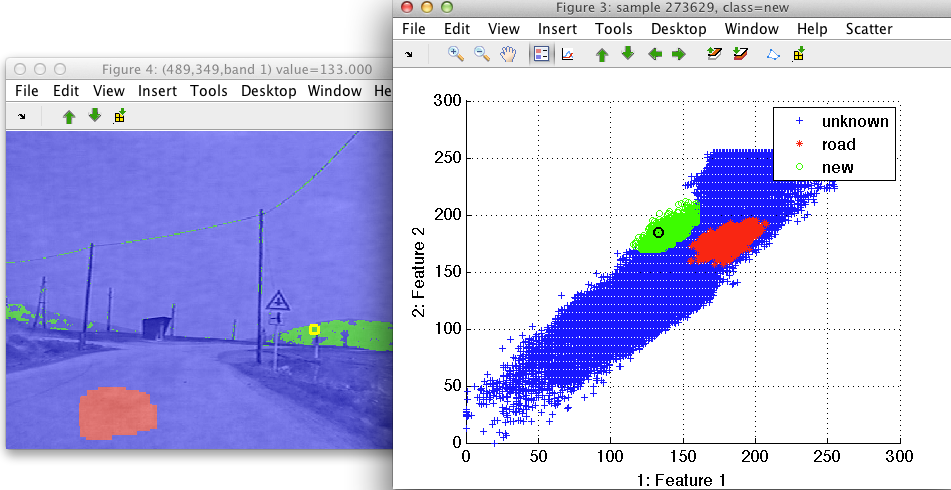
7.10. Connecting sdimage and sdscatter ↩
It is often useful to inspect the connection between image neighborhoods and
the scatter plot. In order to visualize this connection the sdscatter and
sdimage commands can be used together.
We may simply show data set with image data using sdscatter and then
connect the sdimage plot to the scatter figure using the returned figure
handle.
>> data2    %  Created data set data2 in the workspace.
412160 by 3 sddata, 2 classes: 'unknown'(399848) 'road'(12312)

>> h=sdscatter(data2)
h =
     2

>> sdimage(data2,h);
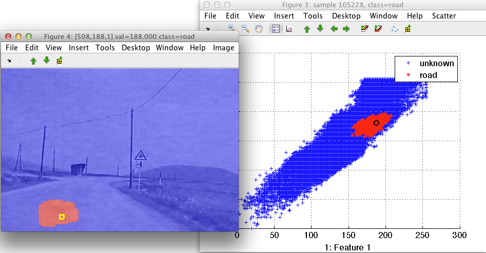
By moving the mouse pointer over the image, we see where the image pixel appears in the feature space. Similarly, moving over the scatter plot shows us the corresponding pixel in the image.
By painting the in the scatter plot, the linked image plot also updates. This helps us to analyze position of specific feature space clusters in image domain:
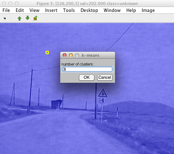
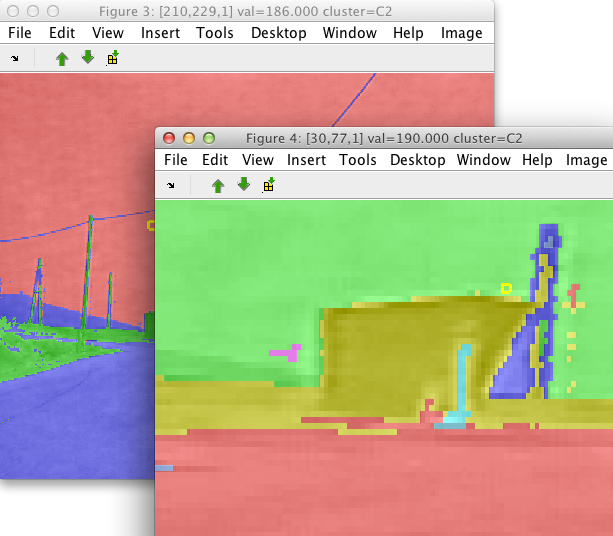
7.11. Clustering image with k-means ↩
One way to quickly group image data is to perform clustering. Using the Cluster with k-means command in Image menu, the data set underlying our image is clustered. The algorithm considers individual pixels as separate data samples and image bands as features.
We are prompted for the desired number of clusters.
We will obtain a new set of image labels called 'cluster' containing classes called 'C1','C2' etc.
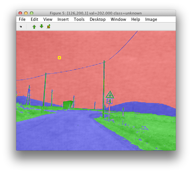
Typical next step is to interpret the clusters. This may be done by assigning meaningful names using the Rename class command.
7.12. Defining connected components ↩
sdimage allows us to define spatially-connected components. This allows
us to quickly access individual objects or regions in an image data set.
The Connected components menu is available only if the current set of
labels contains two or more classes.
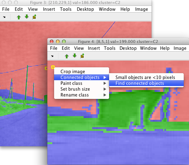
Connected component command processes the current set of labels. For each class, the connected components are found separately.
Small isolated components are joined together into a special class (called 'small objects'). This helps us to quickly remove the noise. By default, objects smaller than 10 pixels are removed. This can be changed by the first item in the Connected components menu. In order to separate all isolated objects, use the value of 1.
When we save the data set back to the Matlab workspace (pressing 's' key),
we can see the 'object' labels. Note that, because we saved the image data
when the 'object' label selected, the resulting data set keeps it as a
current label set. Therefore, we may address it as data2.lab
>> Creating data set data2 in the workspace.
12210 by 3 sddata, 11 'object' groups: [242   160    66  2643   114  6481    72     4  2346    62    20]
>> data2.lab'
 ind name                size percentage
   1 C1-object1           242 ( 2.1%)
   2 C1-object2            10 ( 0.1%)
   3 C1-object3           298 ( 2.6%)
   4 C1-object4            20 ( 0.2%)
   5 C1-object5            66 ( 0.6%)
   6 C1-object6          3805 (33.3%)
   7 C1-small objects      66 ( 0.6%)
   8 C2-object1          4332 (38.0%)
   9 C2-object2            72 ( 0.6%)
  10 C2-small objects       4 ( 0.0%)
  11 C3-object1          2452 (21.5%)
  12 C3-object2            18 ( 0.2%)
  13 C3-object3            14 ( 0.1%)
  14 C3-small objects      14 ( 0.1%)
We can remove the small objects quickly with a regular expression. We simply select all classes, that do not contain the 'small' substring:
>> data2(:,:,'~/small').lab'
 ind name                size percentage
   1 C1-object1           242 ( 2.1%)
   2 C1-object2            10 ( 0.1%)
   3 C1-object3           298 ( 2.6%)
   4 C1-object4            20 ( 0.2%)
   5 C1-object5            66 ( 0.6%)
   6 C1-object6          3805 (33.6%)
   7 C2-object1          4332 (38.2%)
   8 C2-object2            72 ( 0.6%)
   9 C3-object1          2452 (21.6%)
  10 C3-object2            18 ( 0.2%)
  11 C3-object3            14 ( 0.1%)
To define connected components programatically, use the sdsegment
command:
>> s=sdsegment(data2,'minsize',10)