Keywords: detectors, output thresholding
Problem: How to create a detector?
Solution: A step by step example: first split the data into training and test set, second train a model on the desired output, third apply the model to the test set and select the operating point.
A detector is a classifier trained to detect only one class of interest.
>> load fruit  %  Load a three class problem
>> a=sdrelab(a,{'~banana','non-banana'})    %  label all other classes as 'non-banana'
  1: apple  -> non-banana
  2: banana -> banana
  3: stone  -> non-banana
'Fruit set' 260 by 2 sddata, 2 classes: 'banana'(100) 'non-banana'(160)
>> [tr,ts] = randsubset(a,0.5);
>> p=sdmixture(tr('banana'),'n',3)
[class 'banana' EM:.............................. 3 comp]
Mixture of Gaussians pipeline 2x1  one class, 3 components (sdp_normal)
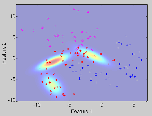
Given a three class problem, we first re-label all classes that are not banana as non-banana. The data is split into training and testing set. This allows for an unbiased selection of the operating point. A mixture of Gaussian is trained only for the class banana. Therefore only that class is passed to the sdmixture routine using the seldat utility. No evidence of the other classes are used to train the model. The scatter plot visualizes the three Gaussians used to model the banana class (with red markers).
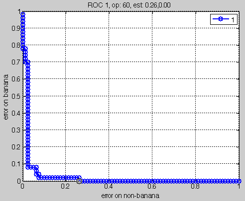
The detector results from thresholding of the outcome of the trained model. In order to choose the appropriate value for the threshold, the ROC analysis is used. The operating point may be chosen by selecting the desired point in the ROC curve plot (number 60, in the example). Its value is then set as default in the ROC object r by pressing the s key on the keyboard.
>> r=sdroc(ts*p)
  1: banana -> banana
  2: non-banana -> non-banana
ROC (130 thr-based op.points, 3 measures), curop: 67
est: 1:err(banana)=0.06, 2:err(non-banana)=0.11, 3:mean-error=0.09
Setting the operating point 60 in sdroc object r
ROC (130 thr-based op.points, 3 measures), curop: 60
est: 1:err(non-banana)=0.26, 2:err(banana)=0.00, 3:mean-error=0.13
>> h=sddrawroc(r)
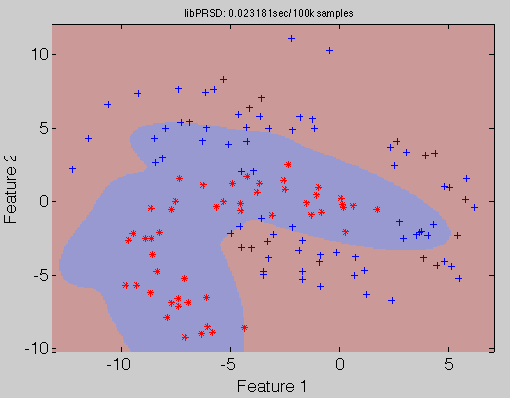
The chosen operating point may now be set in the pipeline. The scatter plot illustrate the decisions of the detector. The banana class is enclosed in the blue region. Note that our detector protects the target banana class from all directions.
>> pd=p*r
sequential pipeline 2x1 'Mixture of Gaussians+Decision'
1 Mixture of Gaussians 2x1 one class, 3 components (sdp_normal)
2 Decision 1x1 thresholding ROC on banana at op 60 (sdp_decide)
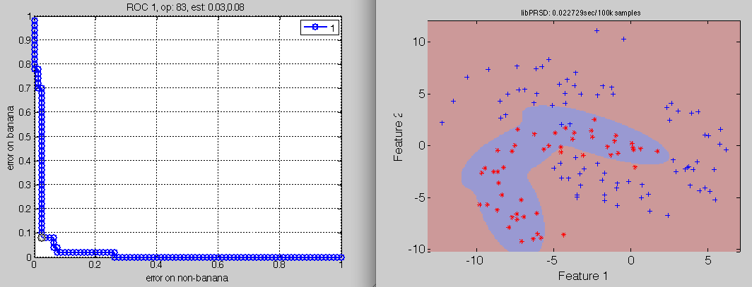
>> sdscatter (ts,pd,'roc',[h])
The scatter plot is linked to the plot with the ROC curve. Hovering the mouse over the operating points will change the detector boundary accordingly. The figure visualizes the decision boundary corresponding to operating point number 83.