
(Please note that starting with perClass 3.x (June 2011), internal parameters of pipelines are not directly accessible)
Problem: How can I optimize classifier on imbalanced problems so that small classes are not misclassified?
Solution: Perform ROC analysis and set operating point delivering better trade-off between class errors.
Sometimes, one of the classes in multi-class problem is much larger than the remaining classes. Classifiers, trained in such imbalanced problem, usually deliver very poor performances with a default decision function. The reason is that the model output of the large class dominates the solution. The default procedure of making decisions assumes that all the classes are equally important which results in high misclassification of small classes.
In this article, we illustrate how to achieve better classifier performance in imbalanced problems using ROC analysis.
17.1. Example of an imbalanced problem ↩
We will use the three-class artificial data set in a 2D feature space. Each of the classes originates from a unimodal Gaussian distribution.
>> load three_class
>> a
'three-class problem' 10800 by 2 sddata, 3 classes: '1'(10000) '2'(400) '3'(400)

>> sdscatter(a)
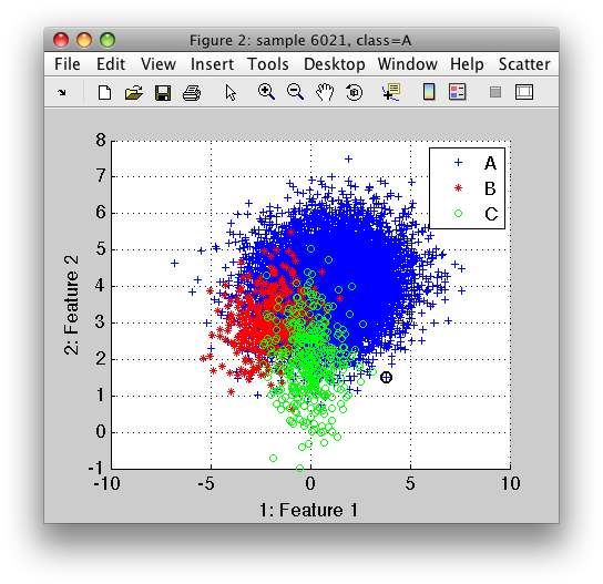
Class A is much larger than classes B and C. All the three classes exhibit high overlap.
Let us first split the data into training and test subsets. We will use the first one for training the model and the second one for estimating the model performance.
>> [tr,ts]=randsubset(a,0.5)
'three-class problem' 5400 by 2 sddata, 3 classes: '1'(5000) '2'(200) '3'(200)
'three-class problem' 5400 by 2 sddata, 3 classes: '1'(5000) '2'(200) '3'(200)
17.2. Training a model ↩
We will use a simple classifier assuming Gaussian densities
sdgauss. Because sdgauss estimates a Gaussian with the full covariance
matrix for each class, the resulting boundary is quadratic.
>> p=sdgauss(tr)
Gaussian model pipeline 2x3  3 classes, 3 components (sdp_normal)
In order to perform decisions, we will first use the common assumption that
each of the classes is equally important. This, so called, default
operating point is equally weighting the per-class outputs of the
statistical model. We may add it to any classifier using the sddecide
function.
>> pd=sddecide(p)
sequential pipeline     2x1 'Gaussian model+Decision'
 1  Gaussian model          2x3  3 classes, 3 components (sdp_normal)
 2  Decision                3x1  weighting, 3 classes, 1 ops at op 1 (sdp_decide)
17.3. Decisions at default operating point ↩
Let us now study the decisions this classifier makes on the test set. We
will use the confusion matrix comparing the true class labels, stored in
ts, with the decisions of the classifier pd:
>> sdconfmat(ts.lab, ts*pd)

ans =

True      | Decisions
Labels    |      A      B      C  | Totals
--------------------------------------------
A         |  4956     14     30   |  5000
B         |   157     41      2   |   200
C         |   119      0     81   |   200
--------------------------------------------
Totals    |  5232     55    113   |  5400
The rows of the matrix correspond to true classes, the columns to the classifier decisions.
We may observe that while the class A is mostly correctly classified, the smaller classes B and C are heavily misclassified. It is even more apparent with the normalized confusion matrix:
>> sdconfmat(ts.lab, ts*pd, 'norm')

ans =

True      | Decisions
Labels    |      A      B      C  | Totals
--------------------------------------------
A         | 0.991  0.003  0.006   | 1.00
B         | 0.785  0.205  0.010   | 1.00
C         | 0.595  0.000  0.405   | 1.00
For class B, we achieve only 20% and for class C 40% performance!
Let us draw this solution in a feature space so we may understand it better.
>> sdscatter(ts,pd)
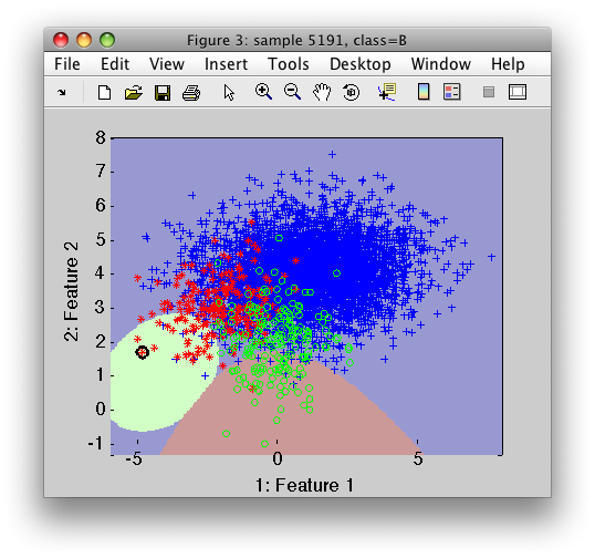
The sample markers in the scatter plot show the ground truth labels in our test set. In the backdrop of the scatter plot, we may see the classifier decisions.
We may note, that the small classes are retracted from the are of overlap which causes the large errors.
The decision function uses a weight vector for each of the three model outputs. The default equal values of the weights let the large class dominate the solution.
17.4. Adjusting the operating point using ROC analysis ↩
In this section, we will show how to find more appropriate weighting of
per-class outputs of our trained model p not sacrificing the examples in
small classes. This is achieved using the ROC analysis approach.
The first step to perform ROC analysis is estimating soft outputs of our trained model on our test set. The soft outputs are the values estimated per class for each test sample.
>> out=ts*p
5400 by 3 sddata, 3 classes: 'A'(5000) 'B'(200) 'C'(200)
The data set out contains soft output of our Gaussian model, namely the
class-conditional densities. The values for the first ten samples in the
test set:
>> +out(1:10)

ans =

0.0196    0.0000    0.0000
0.0127    0.0001    0.0000
0.0770    0.0013    0.0011
0.0166    0.0040    0.0028
0.0770    0.0011    0.0017
0.0663    0.0000    0.0000
0.0614    0.0002    0.0002
0.0542    0.0002    0.0002
0.0242    0.0007    0.0052
0.0880    0.0001    0.0005
To perform ROC analysis, we will simply pass the soft output data set into
the sdroc function:
>> r=sdroc(out)
..........
ROC (2000 w-based op.points, 4 measures), curop: 4
est: 1:err(A)=0.20, 2:err(B)=0.17, 3:err(C)=0.19, 4:mean-error=0.19
The object r, returned by sdroc, contains a set of operating
points and for each point the corresponding performances estimated from the
test set. In this example, the ROC optimizer returned a set of 2000
operating points (weight vectors) and estimated default measures i.e. the
per-class errors and the mean error.
The sdroc object always selects one of the operating points as
current (here the point number 4). By default, the ROC optimizer selects
the point minimizing the mean error over classes. Because the mean error
over classes averages the three per-class errors with equal weights,
optimizing this measure will directly give us a better solution in an
imbalanced situation.
To perform decision at the current operating point of r, we provide it as
the second parameter of sddecide:
>> sdconfmat(ts.lab, ts*sddecide(p,r))

ans =

 True      | Decisions
 Labels    |      A      B      C  | Totals
--------------------------------------------
 A         |  3997    585    418   |  5000
 B         |    15    166     19   |   200
 C         |    15     23    162   |   200
--------------------------------------------
 Totals    |  4027    774    599   |  5400

>> sdconfmat(ts.lab, ts*sddecide(p,r),'norm')

ans =

 True      | Decisions
 Labels    |      A      B      C  | Totals
--------------------------------------------
 A         | 0.799  0.117  0.084   | 1.00
 B         | 0.075  0.830  0.095   | 1.00
 C         | 0.075  0.115  0.810   | 1.00
We can observe that the operating point, found by ROC analysis, results in 80% performance for each class.
17.5. Accessing the weights of the optimized operating point ↩
We may access the complete set of operating points inside the ROC object
r using:
>> r.ops
Weight-based operating set (2000 ops, 3 classes) at op 4
To access only the current one, we use:
>> r.ops(r.curop)
Weight-based operating point,3 classes,[1.17,22.28,...]
Finally, the weights (data) of the operating point are:
>> r.ops(r.curop).data

ans =

1.1732   22.2837   23.4927
Note, that the output of the large class A is played down by this weighting while the outputs of the two smaller classes are emphasized.
17.6. ROC analysis with specific performance measures ↩
Often, we need to consider different performance measures than the default class error rates. We may specify these using the 'measures' option. We need to construct a cell-array with names of the measures followed by parameters. For example, if we want to estimate precision, we will need to specify also the class of interest:
>> M={'precision','A','TPr','A','precision','B','TPr','B','precision','C','TPr','C'};
Using the 'ops' option, we only re-estimate the measures at the set of
operating point in r:
>> r2=sdroc(out,'ops',r.ops,'measures',M)
ROC (2000 w-based op.points, 7 measures), curop: 4
est: 1:precision(A)=0.99, 2:TPr(A)=0.80, 3:precision(B)=0.21, 4:TPr(B)=0.83, 5:precision(C)=0.27, 6:TPr(C)=0.81, 7:mean-error=0.19
Note that our solution suffers from low precision on classes B and C because it was minimizing the mean error and thus, indirectly, the performances.
We may visualize the interactive ROC plot using sdscatter command:
>> sdscatter(ts,sddecide(p,r2),'roc',r2)
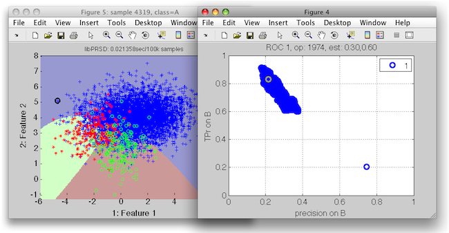
Different combinations of measures in the plot may be selected by the cursor keys.
If you are interested only in visualizing ROC plot, not the scatter, use
the sddrawroc function.
Lets say our main interest is a high-precision solution on class B. We will, therefore look at the trade-off between precision and recall (TPr) on this class. Note that in our ROC object, we do not have any operating points for precision on B higher that 40%. It is because the automatic ROC optimizer gave us only a subset of points with low mean errors.
We may, therefore, estimate ROC again generating a large set of operating points. To keep things simple, we may construct the candidate operating points randomly. We need the weights matrix and the class list specifying the class order:
>> ops=sdops('w',rand(10000,3),tr.lab.list)
Weight-based operating set (10000 ops, 3 classes) at op 1

>> r3=sdroc(out,'ops',ops,'measures',M)
ROC (10000 w-based op.points, 7 measures), curop: 4186
est: 1:precision(A)=0.99, 2:TPr(A)=0.78, 3:precision(B)=0.20, 4:TPr(B)=0.86, 5:precision(C)=0.27, 6:TPr(C)=0.80, 7:mean-error=0.19

>> sdscatter(ts,sddecide(p,r3),'roc',r3)
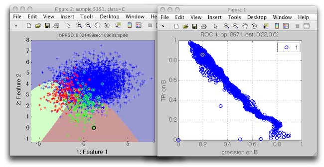
We can see that our new ROC contains also solutions with higher precisions on B.
Finally, we will show how to select an operating point using a specific
performance constrain. For example, we may wish to reach at least 60% of
precision on B. We can apply such constrain with the constrain
method:
>> r4=constrain(r3,'precision(B)',0.6)
ROC (4414 w-based op.points, 7 measures), curop: 4100
est: 1:precision(A)=0.98, 2:TPr(A)=0.88, 3:precision(B)=0.60, 4:TPr(B)=0.39, 5:precision(C)=0.22, 6:TPr(C)=0.90, 7:mean-error=0.28
The resulting classifier sacrifices some TPr to allow for higher precision:
>> sdconfmat(ts.lab, ts*sddecide(p,r4))

ans =

 True      | Decisions
 Labels    |      A      B      C  | Totals
--------------------------------------------
 A         |  4388     50    562   |  5000
 B         |    67     78     55   |   200
 C         |    19      2    179   |   200
--------------------------------------------
 Totals    |  4474    130    796   |  5400
This concludes our example.