perClass Documentation
version 5.4 (7-Dec-2018)

kb30: How to extract image features at multiple scales

Published on: 29-jul-2014

perClass version used: 4.3 (26-may-2014)

Problem: How to combine image features extracted at different scales?

Solution: Use a simple syntax to work with a subset of pixels represented at all scales.

30.1. Introduction ↩

When classifying images, it is useful to extract features at different scales. While small scales describe object details, larger ones capture bigger structures.

Typically, we do not know which specific scale is optimal for our problem. Therefore, we need to compute features at multiple scales and combine them into one data set. With feature selection or extraction methods, we may derive a scale subset useful for our problem.

In this example, we demonstrate how to combine multi-scale features into one data set.

30.2. Computing image features at multiple scales ↩

Local image features, extracted from a square sliding window may be computed with perClass sdextract command.

Let us create an image data set loading the dice image from data sub-directory of perClass distribution:

>> a=sdimage('dice01.jpg','sddata')
101376 by 3 sddata, class: 'unknown'

The dice01.jpg image is loaded with Matlab imread command and reshaped into sddata object a. Each pixel becomes one data sample and is represented by the three features (R, G, and B).

We set the feature labels so that we may use the channel names:

>> a.featlab=sdlab('R','G','B')
101376 by 3 sddata, class: 'unknown'

To visualize our image, use sdimage command:

>> sdimage(a)

ans =

 1

Dice RGB image showing first band.

30.3. Constructing gray channel ↩

As we wish to work with a single gray-level channel, we create a new data set gray fusing the information in the R,G, and B channels, respectively.

One way is to use setdata method to provide a new data matrix, weighting the R, G and B channels:

>> gray=setdata( a, 0.29*+a(:,'R') + 0.587*+a(:,'G') + 0.11*+a(:,'B') )
101376 by 1 sddata, class: 'unknown'

Note the +a(:,'R') syntax that returns raw data matrix for the specified channel.

An alternative is to create an affine projection pipeline and apply it to the data set a:

>> p=sdaffine([0.29 0.587 0.11]',0)
Affine projection pipeline 3x1  

>> gray=a*p
101376 by 1 sddata, class: 'unknown'

30.4. Smoothing image with Gaussian kernel ↩

We will now smooth the image with Gaussian kernel to access image information at larger scale:

>> g=sdextract(gray,'region','gauss','sigma',2,'block',15)
block: 15, sigma: 2.0 yields kernel coverage 100.0%
92612 by 1 sddata, class: 'unknown'

Note, that we specify both the filter sigma and the block size and receive a message computing the coverage of our Gaussian in the selected sliding window (for details see documentation)

It is important to note, that perClass computes region features only in sliding windows that fully cover existing image data. Therefore, the number of samples in the extracted data set g is smaller that in the original gray image.

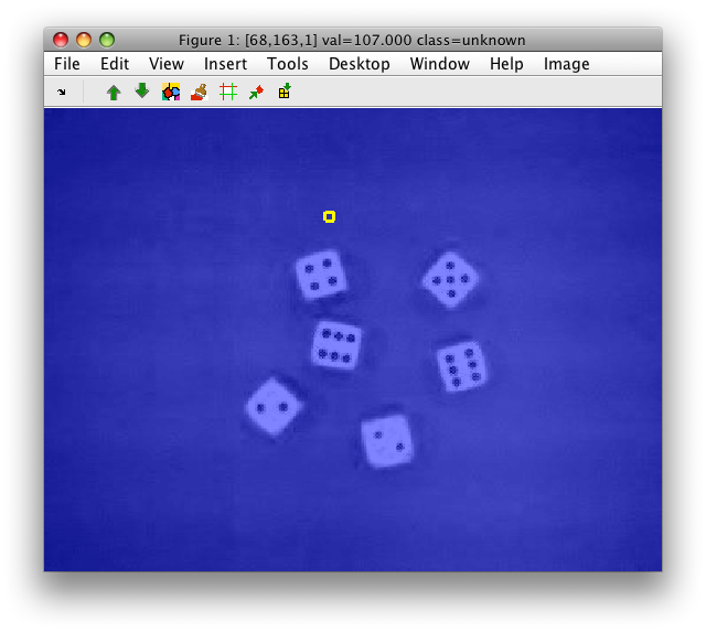
When we visualize the image g, we will notice the border along the image edges where the Gaussian kernel could not be computed.

>> sdimage(g)

ans =

 2

Visualizing image features extracted at scale

30.5. Concatenating images at different scales ↩

The original image data set gray and Gaussian-smoothed image g contain different number of samples:

>> gray
101376 by 1 sddata, class: 'unknown'
>> g
92612 by 1 sddata, class: 'unknown'

Therefore, we cannot simply horizontally concatenate them:

>> data=[gray g]
??? Error using ==> sddata.horzcat at 56
Sample sizes do not match

What we can do, however, is to concatenate subset of pixels represented by both data sets.

perClass 4.3 introduces a simple syntax to find a subset of pixels represented in two image sets:

>> sub=gray(g)
92612 by 1 sddata, class: 'unknown'

The data set sub is created as a subset of data set gray with pixels present both in gray and g.

We can now simply write:

>> data=[sub g]
92612 by 2 sddata, class: 'unknown'

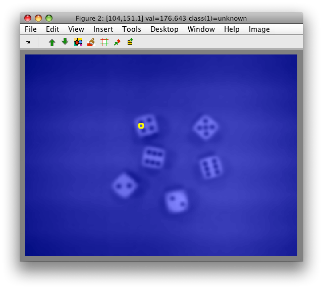
The resulting data set data is an image with two bands. You may visualize it with:

>> sdimage(data)

Flip between the two bands with up/down cursor keys or via toolbar buttons.

To show both bands in one image, we open two separate figures:

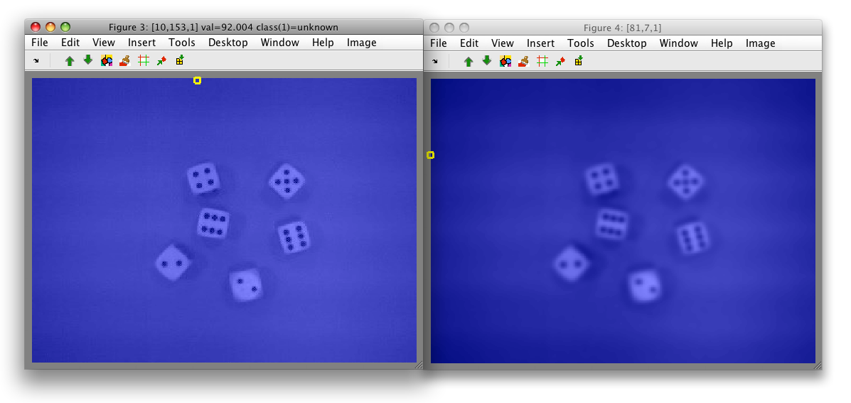
Fusion of image features at different scales.

Note, that both figures show the identical gray border without data. This is because the new data set data only contains pixels represented in both original images.

30.6. Fusing images at multiple scales ↩

If we wish to concatenate images at multiple scales, we simply use preserve only pixels available in the band with largest scale.

For example, say we compute another Gaussian smoothed image, now with sigma of 5.0 in 31x31 windows:

>> g2=sdextract(gray,'region','gauss','sigma',5,'block',31)
block: 31, sigma: 5.0 yields kernel coverage 99.6%
83076 by 1 sddata, class: 'unknown'

The concatenation would then be:

>> data=[gray(g2) g(g2) g2]
83076 by 3 sddata, class: 'unknown'

Both, the gray original image and smaller-scale g image need to be sub-sampled preserving only the pixels available in g2.

30.7. Passing labels from multi-scale to the original image ↩

When working with data sets containing image features at multiple scales, we often face the task of passing the image labels back to the original image.

For example, we may use the concatenated data set data from the example above to define dice labels by clustering.

Open the image view:

>> close all
>> sdimage(data)

Select 'Cluster with k-means' from Image menu (or press 'k').
Fill the desired number of clusters, say 3 and press OK.

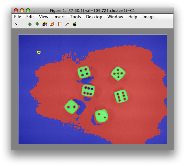
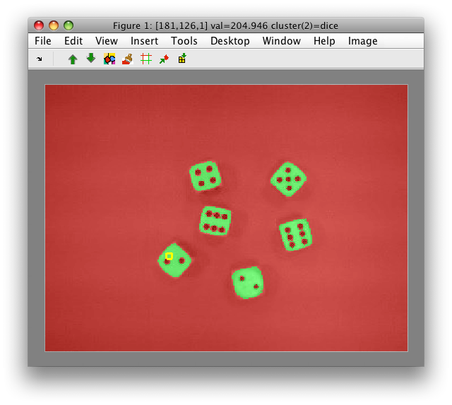
Clustering of image data set with multiple scales.

The derived cluster labels are C1,C2 and C3. We will assign them meaningful names by the rename command. Press 'r' when hovering with the mouse over specific region and use class such as names 'dice' and 'back'. When you provide the same class name 'back' to the two background regions, they will be merged.

Image labels defined by renaming cluster names.

Save the labels into Matlab workspace with 'Create current labels in workspace' command. use L as the name of new label object

>> Creating label set L in the workspace.
sdlab with 83076 entries, 2 groups: 'back'(79736) 'dice'(3340)

The original image set a contains more pixels than the merged set data:

>> data
83076 by 3 sddata, class: 'unknown'
>> a
101376 by 3 sddata, class: 'unknown'

We may assign the labels L to a with:

>> a(data).lab=L
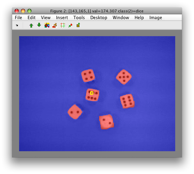
101376 by 3 sddata, 3 classes: 'unknown'(18300) 'back'(79736) 'dice'(3340) 

>> sdimage(a)

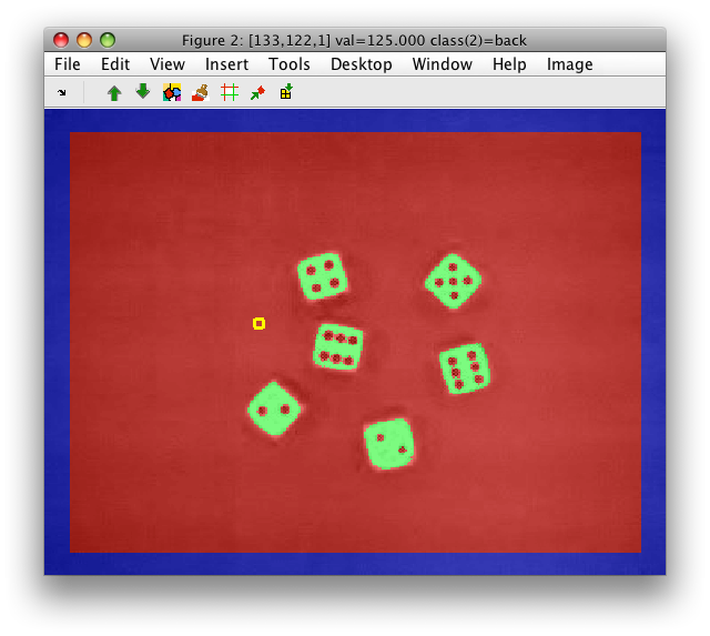
Labels filled in the original image.

We have now passed the labels to the original image. Note, that apart of 'dice' and 'back' classes, there is also the 'unknown' class at the image border.

30.8. Passing labels from the original image to the multi-scale subset ↩

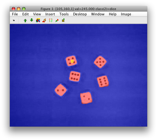
The second use-case is to pass labels from the original image to the multi-scale subset. Say, we have hand-painted labels in the original RGB image a:

>> Creating data set a in the workspace.
101376 by 3 sddata, 2 classes: 'unknown'(97199) 'dice'(4177) 

>> sdimage(a)

ans =

 1

Labels painted on the original RGB image.

Our data set data contains gray-level band and two Gaussian-convolved images at different scales:

>> data
83076 by 3 sddata, class: 'unknown'

>> data.featlab'
   1 Output                  
   2 Output,Gauss(sigma=2.00)
   3 Output,Gauss(sigma=5.00)

To pass the labels a.lab to data, we first create a subset of the original image with pixels that are represented in our multi-scale set data:

>> sub=a(data)
83076 by 3 sddata, 2 classes: 'unknown'(78899) 'dice'(4177)

Now, we can assign the labels of sub into data:

>> data.lab=sub.lab
83076 by 3 sddata, 2 classes: 'unknown'(78899) 'dice'(4177) 

>> sdimage(data)

ans =

 2

Labels assigned to data set with multi-scale features.