
- 16.1. Detection
- 16.1.1. Training a one-class detector
- 16.1.2. Renaming detector decisions
- 16.1.3. Define target class covering all samples in the data
- 16.1.4. Adjusting the amount of rejected target examples
- 16.1.5. Training a two-class detector
- 16.1.6. Repeatable two-class detector
- 16.1.7. Visualizing detector decisions on image data
- 16.1.8. Specifying performance measures for internal ROC
- 16.1.9. Storing confusion matrices in detector ROC
- 16.2. Rejection
16.1. Detection ↩
A detector is a classifier that focuses at one class of interest called the
target class. Detectors may be constructed using the sddetect
command. It takes a data set, the target class and an untrained model as
parameters and returns the trained detector pipeline.
pd = sddetect( data, target_class, model )
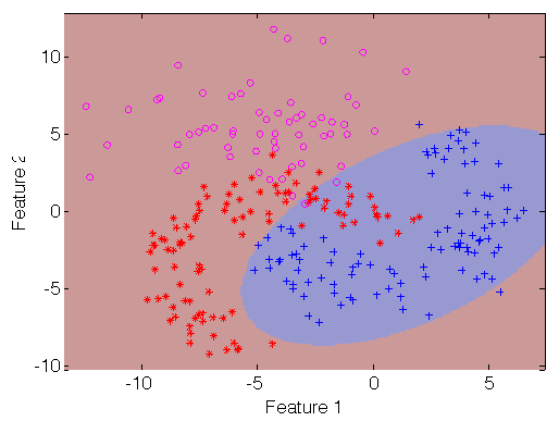
In the example below a Gaussian detector is constructed for the class 'apple' of the fruit data:
>> load fruit
260 by 2 sddata, 3 classes: 'apple'(100) 'banana'(100) 'stone'(60)
>> pd=sddetect(a,'apple',sdgauss)
  1: apple  -> apple
  2: banana -> non-apple
  3: stone  -> non-apple
sequential pipeline       2x1 'Gaussian model+Decision'
 1 Gaussian model          2x1  full cov.mat.
 2 Decision                1x1  ROC thresholding on apple (52 points, current 1)

 >> sdscatter(a,pd)
Detectors are built in two distinct situations:
One-class scenario, where we only have objects of one ('target') class available. The
sddetecttrains the model on the target class and then sets the decision threshold on the model output so that all training objects are accepted. Alternatively, we may opt for rejecting some training objects. Decisions of one-class detectors cannot be adjusted after training.Two-class situation, where we have available both target and non-target examples. The
sddetecttrains the model on target class and then estimates ROC characteristic using both target and non-target data. The performance of the two-class detector can be adjusted any time by changing the ROC decision trade-off.
16.1.1. Training a one-class detector ↩
Imagine, we have a fruit problem with existing apple, banana and stone examples and we want to build one-class detector for apple class.
>> load fruit
>> a
'Fruit set' 260 by 2 sddata, 3 classes: 'apple'(100) 'banana'(100) 'stone'(60)
Although we have a three-class problem, we will build here a one-class detector by using only a single class:
>> a(:,:,'apple')
'Fruit set' 100 by 2 sddata, class: 'apple'
We build a detector on 'apple' using Parzen model:
>> pd=sddetect( a(:,:,'apple') ,'apple',sdparzen)
...sequential pipeline       2x1 'Parzen model+Decision'
 1 Parzen model            2x1  100 prototypes, h=0.6
 2 Decision                1x1  threshold on 'apple'
On a confusion matrix, we may see that our detector fully accepts the
apples on the training set a:
>> sdconfmat(a.lab,a*pd)

ans =

 True      | Decisions
 Labels    |   apple  non-ap  | Totals
---------------------------------------
 apple     |    100       0   |    100
 banana    |      6      94   |    100
 stone     |      0      60   |     60
---------------------------------------
 Totals    |    106     154   |    260
To reject more training examples, you may use the 'reject' option.
16.1.2. Renaming detector decisions ↩
The one-class detector in previous section yields two decisions defined in the detector list:
>> pd.list
sdlist (2 entries)
 ind name
   1 apple
   2 non-apple
By default, the non-target class is named by adding 'non-' prefix to the
target class name. We may change the names of eventual target and
non-target decisions by the corresponding sddetect options:
>> pd=sddetect(a(:,:,'apple'),'apple',sdparzen,'non-target','others')
...sequential pipeline       2x1 'Parzen model+Decision'
 1 Parzen model            2x1  100 prototypes, h=0.6
 2 Decision                1x1  threshold on 'apple'

>> pd.list
sdlist (2 entries)
 ind name
   1 apple
   2 others
16.1.3. Define target class covering all samples in the data ↩
Sometimes, we build a detector for a concept that is not directly labeled in our data set. For example, in the fruit problem, we have apples, bananas and stones labeled but may want to create a detector for all fruit.
If we specify, in sddetect, a target class name that is not present in
the provided dataset, this class will be used for all samples and one-class
detector is built.
>> a
'Fruit set' 260 by 2 sddata, 3 classes: 'apple'(100) 'banana'(100) 'stone'(60)
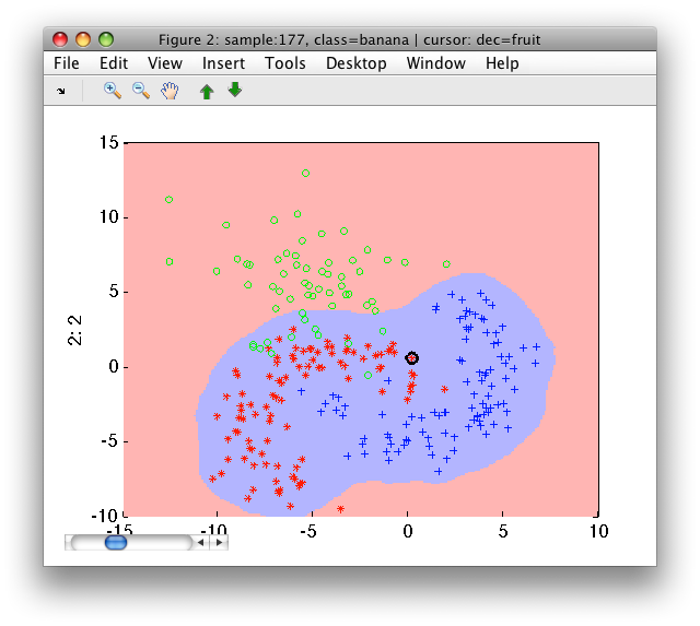
To build a one-class fruit detector, we create a data subset with apple and banana samples:
>> b=a(:,:,{'apple','banana'})
'Fruit set' 200 by 2 sddata, 2 classes: 'apple'(100) 'banana'(100)
We build a Parzen detector on b calling the target class 'fruit'. Because
'fruit' is not available in the b.list, all provided samples are used to
build one-class model and called 'fruit':
>> pd=sddetect(b,'fruit',sdparzen)
....sequential pipeline       2x1 'Parzen model+Decision'
 1 Parzen model            2x1  200 prototypes, h=0.6
 2 Decision                1x1  threshold on 'fruit'

>> pd.list
sdlist (2 entries)
 ind name
   1 fruit
   2 non-fruit

>> sdconfmat(a.lab,a*pd)

ans =

 True      | Decisions
 Labels    |   fruit  non-fr  | Totals
---------------------------------------
 apple     |    100       0   |    100
 banana    |    100       0   |    100
 stone     |     13      47   |     60
---------------------------------------
 Totals    |    213      47   |    260

>> sdscatter(a,pd)
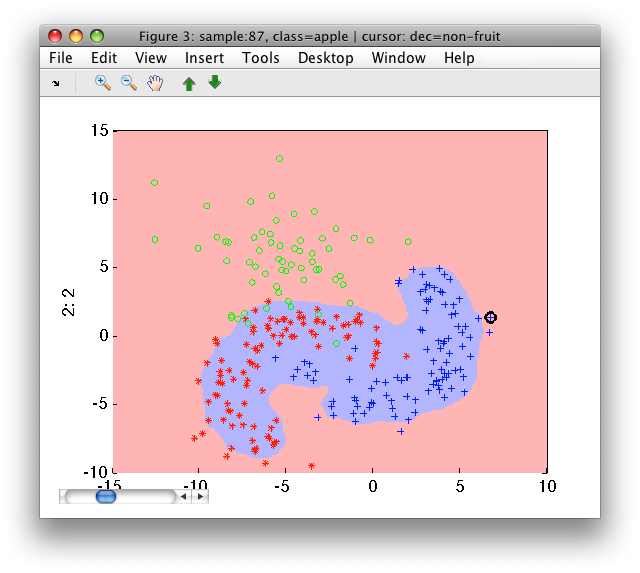
16.1.4. Adjusting the amount of rejected target examples ↩
By default, one-class detectors accept all training targets. However,
sometimes we may wish to actually reject some target examples. For example,
our data set may contain outliers or we may wish to create a tighter
one-class description. The sddetect 'reject' option allows us to adjust
the number of rejected targets either by fraction or by number of samples
rejected.
>> pd=sddetect(b,'fruit',sdparzen,'reject',10)
....sequential pipeline       2x1 'Parzen model+Decision'
 1 Parzen model            2x1  200 prototypes, h=0.6
 2 Decision                1x1  threshold on 'fruit'

>> sdconfmat(a.lab,a*pd)

ans =

 True      | Decisions
 Labels    |   fruit  non-fr  | Totals
---------------------------------------
 apple     |     95       5   |    100
 banana    |     95       5   |    100
 stone     |      7      53   |     60
---------------------------------------
 Totals    |    197      63   |    260

>> sdscatter(a,pd)
Instead of the number of rejected targets, we may specify fraction of the trainig set to be rejected:
>> pd=sddetect(b,'fruit',sdparzen,'reject',0.03)
....sequential pipeline       2x1 'Parzen model+Decision'
 1 Parzen model            2x1  200 prototypes, h=0.6
 2 Decision                1x1  threshold on 'fruit'
>> sdconfmat(a.lab,a*pd)

ans =

 True      | Decisions
 Labels    |   fruit  non-fr  | Totals
---------------------------------------
 apple     |     98       2   |    100
 banana    |     96       4   |    100
 stone     |      8      52   |     60
---------------------------------------
 Totals    |    202      58   |    260
16.1.5. Training a two-class detector ↩
A two-class detector is build other classes than the target class are
present in the data set passed to sddetect.
The model is trained on the target class and ROC analysis is performed using both target and non-target classes. Therefore, we may adjust the trained detector later:
>> load fruit
260 by 2 sddata, 3 classes: 'apple'(100) 'banana'(100) 'stone'(60)

>> pd=sddetect(a,'apple',sdgauss)
  1: apple  -> apple
  2: banana -> non-apple
  3: stone  -> non-apple
sequential pipeline       2x1 'Gaussian model+Decision'
 1 Gaussian model          2x1  full cov.mat.
 2 Decision                1x1  ROC thresholding on apple (52 points, current 1)
Because we specify to build a detector on 'apple', the two other classes
('banana' and 'stone') are considered non-target. The sddetect function
displays the renaming rules.
The ROC object is available in the pd.roc field:
>> pd.roc
ROC (52 thr-based op.points, 3 measures), curop: 1
est: 1:err(apple)=0.00, 2:err(non-apple)=0.19, 3:mean-error=0.09
We may visualize the ROC with sddrawroc directly using the pipeline object pd:
>> sddrawroc(pd)
We may choose a different op.point and save it back to the pd object
(with 'Store to workspace' toolbar button or pressing 's' key):
>> Setting the operating point 31 in sdppl object pd
sequential pipeline       2x1 'Gaussian model+Decision'
 1 Gaussian model          2x1  full cov.mat.
 2 Decision                1x1  ROC thresholding on apple (52 points, current 31)
16.1.6. Repeatable two-class detector ↩
When we train a two-class detector twice on the same data, we receive slightly different resuts:
>> pd=sddetect(a,'apple',sdgauss)
  1: apple  -> apple
  2: banana -> non-apple
  3: stone  -> non-apple
sequential pipeline       2x1 'Gaussian model+Decision'
 1 Gaussian model          2x1  full cov.mat.
 2 Decision                1x1  ROC thresholding on apple (52 points, current 1)
>> sdconfmat(a.lab,a*pd)

ans =

 True      | Decisions
 Labels    |   apple  non-ap  | Totals
---------------------------------------
 apple     |     97       3   |    100
 banana    |     20      80   |    100
 stone     |      2      58   |     60
---------------------------------------
 Totals    |    119     141   |    260

>> pd=sddetect(a,'apple',sdgauss)
  1: apple  -> apple
  2: banana -> non-apple
  3: stone  -> non-apple
sequential pipeline       2x1 'Gaussian model+Decision'
 1 Gaussian model          2x1  full cov.mat.
 2 Decision                1x1  ROC thresholding on apple (52 points, current 1)
>> sdconfmat(a.lab,a*pd)

ans =

 True      | Decisions
 Labels    |   apple  non-ap  | Totals
---------------------------------------
 apple     |     99       1   |    100
 banana    |     20      80   |    100
 stone     |      2      58   |     60
---------------------------------------
 Totals    |    121     139   |    260
It is because, internally, sddetect splits the provided data set a
randomly into two parts. One is used for building the target model, the
other for ROC analysis. As with any other perClass routine performing
internal data split, we have full control of this mechanism.
Firstly, we may fix the Matlab random number generator before training the
sddetect to receive identical output:
>> rand('state',42); pd=sddetect(a,'apple',sdgauss,'nodisplay');
>> sdconfmat(a.lab,a*pd)

ans =

 True      | Decisions
 Labels    |   apple  non-ap  | Totals
---------------------------------------
 apple     |     95       5   |    100
 banana    |     19      81   |    100
 stone     |      1      59   |     60
---------------------------------------
 Totals    |    115     145   |    260
Secondly, we may split the data set ourselves and pass the subset to train the model and the subset to perform ROC manually with 'test' option:
>> [tr,val]=randsubset(a,50)
'Fruit set' 150 by 2 sddata, 3 classes: 'apple'(50) 'banana'(50) 'stone'(50)
'Fruit set' 110 by 2 sddata, 3 classes: 'apple'(50) 'banana'(50) 'stone'(10)
>> pd=sddetect(tr,'apple',sdgauss,'nodisplay','test',val);
>> sdconfmat(val.lab,val*pd)

ans =

 True      | Decisions
 Labels    |   apple  non-ap  | Totals
---------------------------------------
 apple     |     49       1   |     50
 banana    |     11      39   |     50
 stone     |      0      10   |     10
---------------------------------------
 Totals    |     60      50   |    110
The ROC was estimated from the val data set. Therefore, the error
measures stored in ROC object match our confusion matrix:
>> pd.roc
ROC (110 thr-based op.points, 3 measures), curop: 49
est: 1:err(apple)=0.02, 2:err(non-apple)=0.18, 3:mean-error=0.10
>> 1/50   %  error on apple

ans =

0.0200

>> 11/(50+10)  %  error on non-apple (banana + stone)

ans =

0.1833
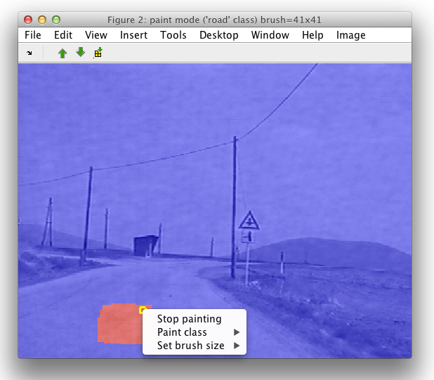
16.1.7. Visualizing detector decisions on image data ↩
sdimage may visualize decisions of any classifier pipeline trained on
image data. We may also inspect decisions in an image at different
operating points.
We save the hand-painted road labels into data2 data set:
>> data2
412160 by 3 sddata, 2 classes: 'unknown'(399848) 'road'(12312)
Now we may train the road detector. We use a subset of 500 pixels for road sign background classes and train the detector:
>> b=randsubset(data2,500)
1000 by 3 sddata, 2 classes: 'unknown'(500) 'road'(500)

>> pd=sddetect(b,'road',sdgauss)
  1: unknown -> non-road
  2: road   -> road
sequential pipeline       3x1 'Gaussian model+Decision'
 1 Gaussian model          3x1  full cov.mat.
 2 Decision                1x1  ROC thresholding on road (180 points, current 77)
We can now visualize the detector decisions on another image:
>> im2=imread('roadsign11.bmp');
>> sdimage(im2,pd)
ans =
 3
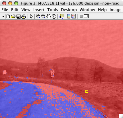
sdimage may visualize both the decisions and the ROC of the detector:
>> sdimage(im2,pd,'roc')
ans =
 1
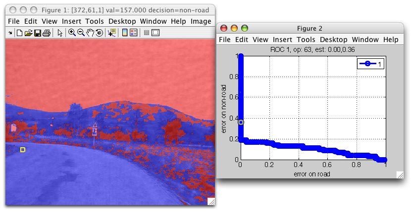
This allows us to interactively analyze detector decisions at different operating points.
16.1.8. Specifying performance measures for internal ROC ↩
When both target and non-target data is available, sddetect estimates ROC
to set the detector operating point. By default, class errors and mean
error over classes are estimated. We may wish to use different,
application-specific measures. This is possible with 'measures' option:
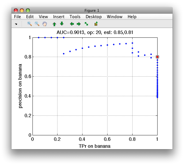
In this example on fruit data, we build Parzen detector on banana and estimate true positive date and precision:
>> pd=sddetect(a,'banana',sdparzen,'measures',{'TPr','banana','precision','banana'})
...  1: apple  -> non-banana
  2: banana -> banana
  3: stone  -> non-banana
sequential pipeline       2x1 'Parzen model+Decision'
 1 Parzen model            2x1  80 prototypes, h=0.6
 2 Decision                1x1  ROC thresholding on banana (52 points, current 52)

>> sddrawroc(pd)
16.1.9. Storing confusion matrices in detector ROC ↩
By default, detector does not store confusion matrices in the internal ROC object. It may be useful to store condution matrices in order to visualize them or use cost-sensitive optimization to set operating point later. This is possible using the 'confmat' option.
16.2. Rejection ↩
Rejection refers to the choice we make not to assign the data sample to any of the learned classes. The sample may be either discarded or passed for further processing by a different system or human expert.
perClass supports both types of rejection:
- Distance-based rejection where we discard data samples far away from the learned class distributions. This rejection scheme helps us to protect against outliers
- Rejection close to the decision boundary where we reject data samples that fall into the area of class overlap and hence are likely to be misclassified.
The fastest way to add a reject option to a trained pipeline is to use
sdreject command. Alternatively, we may construct the full reject curve
from classifier soft outputs with sdroc. This is useful to investigate
performances at a set of reject thresholds.
Technically, the reject option for pipelines with a single soft-output is implemented by a thresholding-based operating point. For discriminants, the reject threshold is added to the weighting-based operating point. This allows us to model both rejection types depending on the type of the soft output used. If the soft output was normalized with respect to all classes, the rejection operates close to the boundary. Without normalization, the rejection discard outliers.
16.2.1. Adding reject option to a trained pipeline ↩
sdreject command adds the reject option to a trained pipeline. We need to
provide it with the pipeline, data set used for computing the rejection
threshold. By default, sdreject sets the threshold to reject 1% of
provided data samples.
>> b
'Fruit set' 1334 by 2 sddata, 2 classes: 'apple'(667) 'banana'(667)

>> p=sdmixture(b)
[class 'apple' initialization: 4 clusters  EM:.............................. 4 comp]
[class 'banana' initialization: 4 clusters  EM:.............................. 4 comp]
Mixture of Gaussians pipeline 2x2  2 classes, 8 components (sdp_normal)

>> pr=sdreject(p,b)
sequential pipeline     2x1 'Mixture of Gaussians+Decision'
 1  Mixture of Gaussians    2x2  2 classes, 8 components (sdp_normal)
 2  Decision                2x1  weight+reject, 3 decisions, 1 ops at op 1 (sdp_decide)

>> sdscatter(b,pr)
In order to adjust the rejected data fraction, use the 'reject' option:
>> pr=sdreject(p,b,'reject',0.2)
sequential pipeline     2x1 'Mixture of Gaussians+Decision'
 1  Mixture of Gaussians    2x2  2 classes, 8 components (sdp_normal)
 2  Decision                2x1  weight+reject, 3 decisions, 1 ops at op 1 (sdp_decide)
>> sdscatter(b,pr)
16.2.2. Reject curve for distance-based rejection ↩
To illustrate distance-based rejection, we will use two-class Higleyman data set and train quadratic discriminant:
>> a
'Highleyman Dataset' 300 by 2 sddata, 2 classes: '1'(154) '2'(146)

>> [tr,ts]=randsubset(a,0.5);
>> p=sdgauss(tr)
Gaussian model pipeline 2x2  2 classes, 2 components (sdp_normal)
We estimate soft outputs on the test set:
>> out=ts*p
'Highleyman Dataset' 150 by 2 sddata, 2 classes: '1'(77) '2'(73)
>> +out(1:5,:)

ans =

0.0747    0.0000
0.1233    0.0036
0.0777    0.0393
0.1121    0.0000
0.1099    0.1760
Note that the soft outputs do not sum to one. That is because sdgauss returns
class conditional densities.
We will now use sdroc command to construct a reject curve at default
operating point. It will add the rejection capability to the operating
point and derive a set of feasible rejection thresholds from the data. In
this example, default operating point (equal class weights) will be used as
a bases for adding reject option:
>> r=sdroc(out,'reject')
ROC (1001 wr-based op.points, 4 measures), curop: 1
est: 1:frac(reject)=0.00, 2:TPr(1)=0.86, 3:TPr(2)=0.97, 4:TPr(reject)=0.00
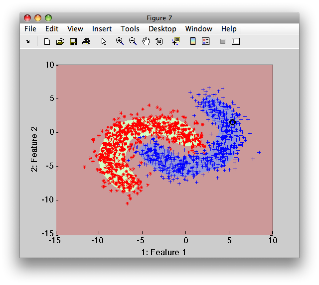
We can visualize the decisions using sdscatter.
>> sdscatter(ts,p*r,'roc',r)
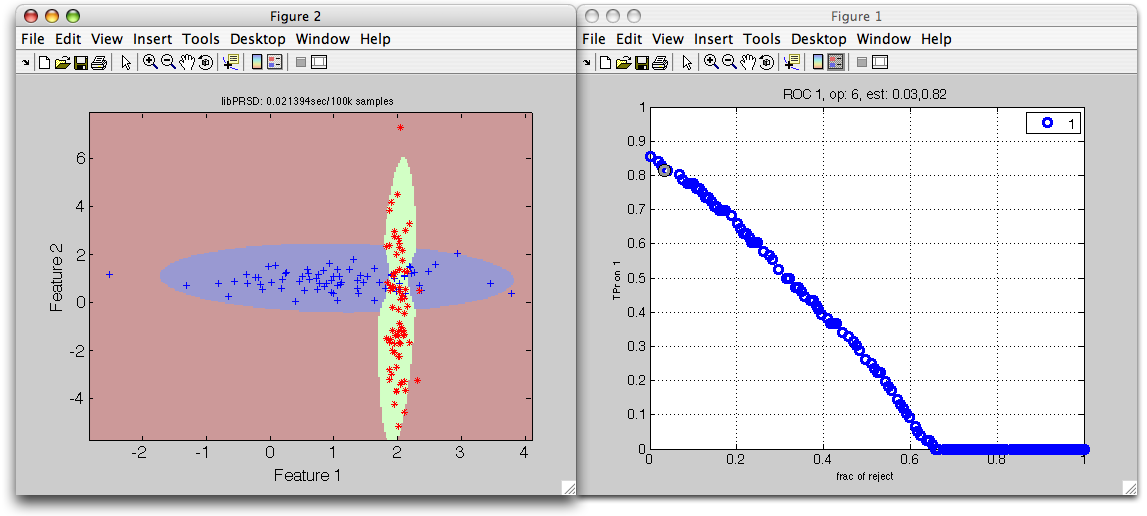
The horizontal axis represents the fraction of rejected objects; vertical the true positive ratio for the first class. By moving out of the default operating point (where rejection is not performed), we can observe how rejection takes place far from both trained distributions.
We can select a specific point by left mouse click and store it back to the
r object by pressing s key. We can now estimate the confusion matrix on
the test set:
>> r=setcurop(r,6); %  Setting the operating point 6 in sdroc object r
ROC (1001 wr-based op.points, 4 measures), curop: 6
est: 1:frac(reject)=0.03, 2:TPr(1)=0.82, 3:TPr(2)=0.95, 4:TPr(reject)=0.00
>> sdconfmat(ts.lab,ts*p*r)

ans =

 True      | Decisions
 Labels    | 1      2      reject  | Totals
--------------------------------------------
 1         |    62     11      3   |    76
 2         |     2     69      2   |    73
--------------------------------------------
 Totals    |    64     80      5   |   149
We can see that the confusion matrix contains the added reject decision.
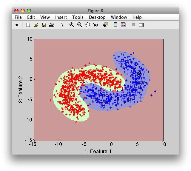
16.2.3. Reject curve for rejection close to the decision boundary ↩
To illustrate the rejection close to the decision boundary, we will continue in the example above. We make a single change in the procedure above: we normalize the model soft outputs to sum to one.
>> p2=sdquadratic(tr)
sequential pipeline     2x2 'Quadratic discr.'
 1  Gauss full cov.         2x2  2 classes, 2 components (sdp_normal)
 2  Output normalization    2x2  (sdp_norm)
>> out2=ts*p2
'Highleyman Dataset' 150 by 2 sddata, 2 classes: '1'(77) '2'(73)
>> +out2(1:5,:)

ans =

1.0000    0.0000
0.9717    0.0283
0.6639    0.3361
1.0000    0.0000
0.3843    0.6157
Note that the classifier outputs are now posterior probabilitites, not densities.
>> r2=sdroc(out2,'reject')
ROC (1001 wr-based op.points, 4 measures), curop: 1
est: 1:frac(reject)=0.00, 2:TPr(1)=0.87, 3:TPr(2)=0.97, 4:TPr(reject)=0.00

>> sdscatter(ts,p*r2,'roc',r2)
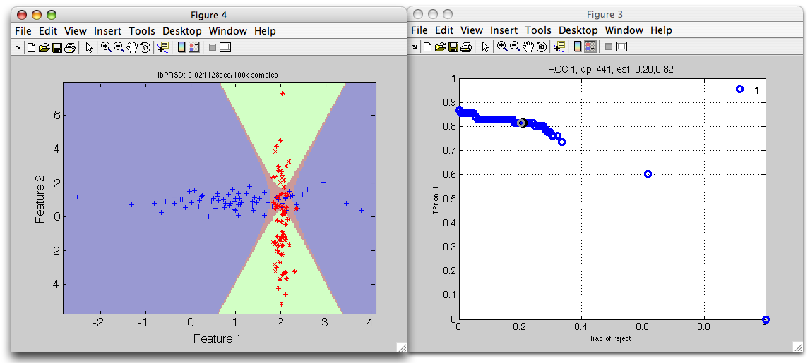
The red reject decision now occupies the area where errors would be highly probably.
16.2.4. Adding reject option to a specific operating point ↩
By default, the reject option will add rejection to a default operating
point (with equal class weights). In order to add the reject option to a
different operating point, we may pass operating set sdops or ROC
object sdroc:
>> a
'Fruit Set', 2000 by 2 sddata with 2 classes: 'apple' (983) 'banana' (1017)
>> p %  trained Parzen classifier
sequential pipeline     2x2 ''
 1  sdp_parzen          2x2  2 classes, 1601 prototypes
>> out=a*p %  soft outputs
'Fruit Set', 2000 by 2 sddata with 2 classes: 'apple' (983) 'banana' (1017)
>> r=sdroc(out) %  standard ROC
ROC (2001 w-based op.points, 3 measures), curop: 1014
est: 1:err(1)=0.02, 2:err(2)=0.02, 3:mean-error [0.50,0.50]=0.02
We will choose a different operating point - e.g. the point 100 where we're not loosing the class 2:
>> r=setcurop(r,100)
ROC (2001 w-based op.points, 3 measures), curop: 100
est: 1:err(1)=0.25, 2:err(2)=0.00, 3:mean-error [0.50,0.50]=0.13
To create a rejection curve starting from this operating point, just pass
the r to the reject option:
>> r2=sdroc(out,'reject',r)
ROC (1001 wr-based op.points, 4 measures), curop: 1
est: 1:frac(reject)=0.00, 2:TPr(1)=0.75, 3:TPr(2)=1.00, 4:TPr(reject)=0.00
The eventual pipeline would be:
>> p2=p*r2
sequential pipeline     2x1 'Parzen+Decision'
 1  Parzen                  2x2  2 classes, 200 prototypes (sdp_parzen)
 2  Decision                2x1  weight+reject, 3 decisions, 1001 ops at op 1 (sdp_decide)
>> p2.list
sdlist (3 entries)
 ind name
   1 1
   2 2
   3 reject