
Keywords: ROC, classifier, cascade of classifiers
Problem: How to tag decisions that are sure (correct) and unsure (may lead to error)?
Solution: Use ROC to choose operating points separating (most probably) correct and unsure decisions.
33.1. Introduction ↩
Imagine, you could set your classifier in such a way that decisions it makes are always correct and all the unsure samples are tagged for further inspection. In this example, we discuss how to achieve this for any two-class classifier accompanied with an ROC characteristic.
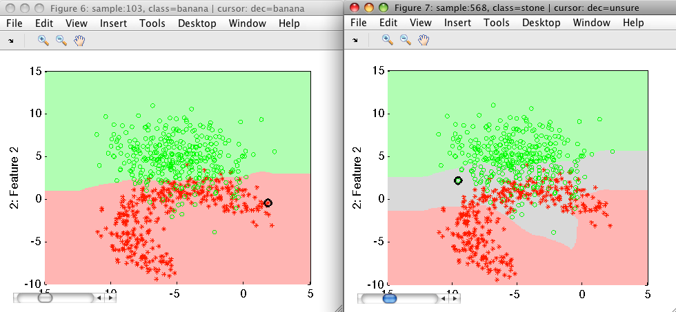
Example on the screenshot below: On the left is a result of a classifier in our two-class problem that makes some errors in the area of overlap. On the right is the solution discussed here where we return two 'sure' decisions that do not suffer from errors and 'unsure' decision denoting the gray-area:
33.2. Motivation ↩
Most of classification problems we're dealing with in practice exhibit some errors. This is due to overlap in the feature space that cannot be mitigated even by the best of models.
Typically, we optimize our classifier with ROC analysis and choose a trade-off aligned with the application requirements. For example, we require at least 95% classifier sensitivity (correct detection of true targets) while minimizing the false positives. With such a solution, we need to live with errors. ROC only helps us to consciously choose which error type(s) we allow and which ones we limit.
Sometimes, however, we may wish to recover all correctly classified samples and tag the remaining, unsure, examples where errors are more likely. This approach is highly desirable if our classifier is followed by another stage. It may be a human sorter who post-processes the difficult cases or other automated system using more sophisticated sensor.
33.3. Preparing data and classifier ↩
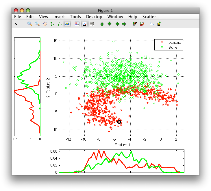
In the first example, we use the fruit data set, namely the banana and stone classes that exhibit some overlap.
>> load fruit_large
>> A=a(:,:,[2 3])
'Fruit set' 1333 by 2 sddata, 2 classes: 'banana'(667) 'stone'(666)

>> sdscatter(A)

ans =

 1
We split the data set into training and test subsets:
>> [tr,ts]=randsubset(A,0.5)
'Fruit set' 666 by 2 sddata, 2 classes: 'banana'(333) 'stone'(333)
'Fruit set' 667 by 2 sddata, 2 classes: 'banana'(334) 'stone'(333)
We train the Parzen classifier on the training part:
>> p=sdparzen(tr)
.......sequential pipeline       2x1 'Parzen model+Decision'
 1 Parzen model            2x2  666 prototypes, h=0.6
 2 Decision                2x1  weighting, 2 classes
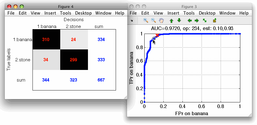
We estimate ROC on the test set and specify our measures of interest, namely the FPr and TPr considering banana as our target class:
>> r=sdroc(ts,p,'measures',{'FPr','banana','TPr','banana'},'confmat')
ROC (468 w-based op.points, 3 measures), curop: 260
est: 1:FPr(banana)=0.14, 2:TPr(banana)=0.98, 3:mean-error=0.08
Note, we have also used the 'confmat' option so that confusion matrices are
stored in the ROC object r.
We can now put together the classifier and ROC into one pipeline...
>> pall=p*r
sequential pipeline       2x1 'Parzen model+Decision'
 1 Parzen model            2x2  666 prototypes, h=0.6
 2 Decision                2x1  ROC weighting, 2 classes, 468 op.points at current 260
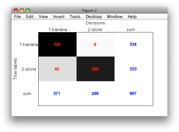
... and visualize the confusion matrix on the test set:
>> sdconfmat(ts.lab,ts*pall,'figure')

ans =

 2
33.4. Inspecting ROC plot ↩
To better understand how our classifier makes decisions we visualize its ROC:
>> sddrawroc(pall)

ans =

 3
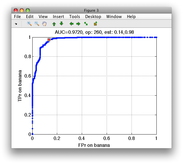
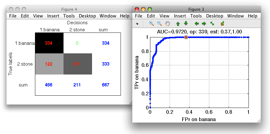
The default operating point is selected so that mean error over classes is minimized. For us, it is interesting to inspect what happens close to the axes in limit situations minimizing one of the errors. We open the confusion matrix by pressing 'c' key on the keyboard. By moving over operating points, we will identify a point where banana decisions (denoted in columns) are all correct.
Similarly, we may choose an operating point where stone decisions will be always correct.
33.5. Putting it all together ↩
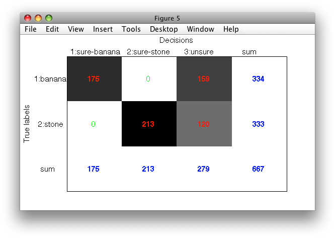
Decisions at both operating points are put together in a function tag_unsure_decisions.m.
As input, it accepts a trained classifier containing ROC, the name of target class, allowed error on target, the name of non-target class and the error on non-target. The function returns a new pipeline separating sure targets, sure non-targets and unsure decisions.
>> pc=tag_unsure_decisions(pall,'banana',0,'stone',0)
sequential pipeline       2x1 'Parzen model+Classifier cascade'
 1 Parzen model            2x2  666 prototypes, h=0.6
 2 Classifier cascade      2x1  2 stages

>> sdconfmat(ts.lab,ts*pc,'figure')

ans =

 5
How do the decisions of our classifier actually look-like?
>> sdscatter(ts,pall)

ans =

 6

>> sdscatter(ts,pc)

ans =

 7
We can see the original classifier on the left and the new one on the right. The gray area corresponds to the unsure decisions. Both banana and stone decisions are perfect on this test set.
33.6. Tuning per-class errors ↩
Sometimes, we may wish to allow some small error for one of the classes. This may help us to find significantly better solution. In our example, we may wish to allow 2% error on banana. This will allow us to recover significantly more stones:
>> pcx=tag_unsure_decisions(pall,'banana',0.02,'stone',0)
sequential pipeline       2x1 'Parzen model+Classifier cascade'
 1 Parzen model            2x2  666 prototypes, h=0.6
 2 Classifier cascade      2x1  2 stages

>> sdconfmat(ts.lab,ts*pcx,'figure')
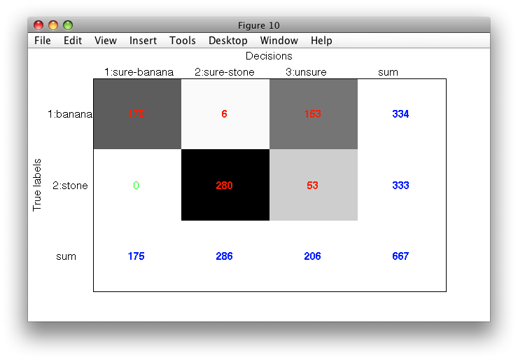
Allowing small error on "sure" class may seem strange at first. However, this strategy is very useful in practice due to probabilistic nature of ROC estimates. We are, of course, removing all mistakes on a specific class only on the test set where ROC was estimated. On a large independent set, we might see slightly different estimates. Allowing small error instead of zero error is often a pragmatic choice.
33.7. Processing also unsure decisions ↩
Finally, we may wish to process also the unsure decisions by the original
classifier. The tag_unsure_decisions.m function does it if we specify
optional process_unsure flag:
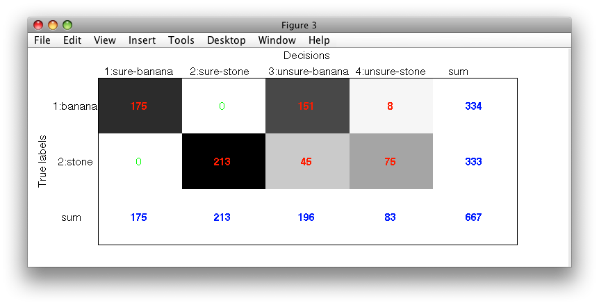
>> pc2=tag_unsure_decisions(pall,'banana',0,'stone',0,1)
  1: banana -> unsure-banana
  2: stone  -> unsure-stone
sequential pipeline       2x1 'Parzen model+Classifier cascade'
 1 Parzen model            2x2  666 prototypes, h=0.6
 2 Classifier cascade      2x1  3 stages

>> sdconfmat(ts.lab,ts*pc2,'figure')

ans =

 3
>> sdscatter(ts,pc2)

ans =

 4
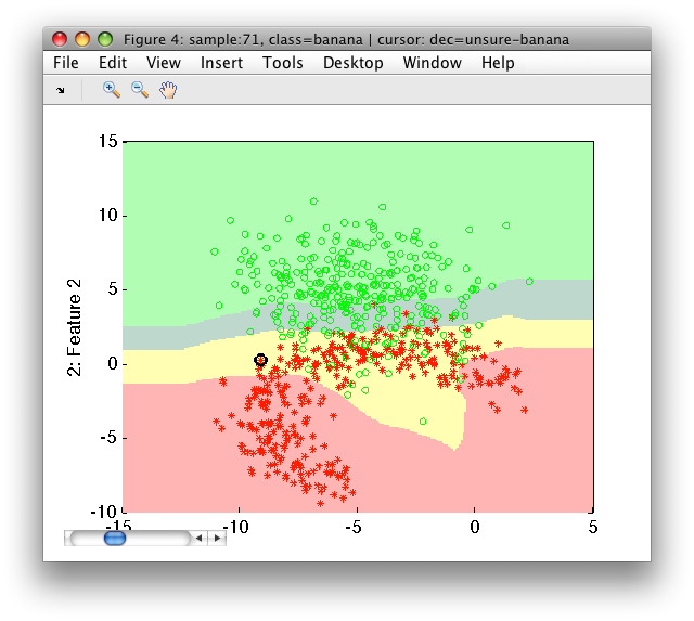
Note, that the gray unsure area from the previous plot is now split into yellow unsure-banana and dark-green unsure-stone areas.
33.8. Conclusions ↩
We have seen how to augment any two-class classifier with ROC to provide additional information if its decisions are sure or unsure. Presented solution is directly applicable to any classifier type (density/distance/confidence) and to arbitrarily-dimensional feature spaces. It can also be directly exported out-of-Matlab and run in a custom application via perClass Runtime. This allows us to directly validate unsure sample tagging. Regarding execution speed, this method does not incur any extra penalty because the model is executed only once on each sample.