
Keywords: support vector machines, LIBSVM, classifier execution
Problem: How to execute support vector classifier trained in LIBSVM using libPRSD?
Solution: Call sdp_svc pipeline constructor and fill in parameters trained by LIBSVM.
Note: Starting with release 2.1, PRSD Studio provides sdsvc command that
encapsulates training of RBF support vector machines in libSVM. See example.
The following example illustrates how may be classifier parameters, trained using external libraries, imported in PRSD Studio and executed using libPRSD library out of Matlab.
PRSD Studio exposes number of pattern recognition algorithms to the user as pipeline actions. For each algorithm, we may construct an execution pipeline directly by supplying its canonical parameters (see function reference for parameters of pipeline actions). Usually, we train the classifiers directly in PRSD Studio. However, we may as well train the algorithm using external tools or libraries as long as we are able to provide its parameters to the pipeline constructor under Matlab.
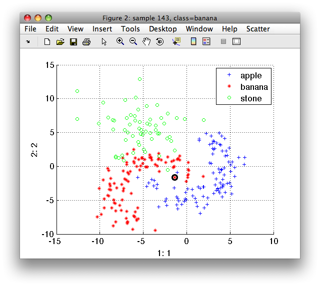
In this example, we use "A simple MATLAB interface" of LIBSVM authors, you can download from here (ver.2.9.1). We use simple 'fruit' data set problem':
>> load fruit
>> a
'Fruit set' 260 by 2 sddata, 3 classes: 'apple'(100) 'banana'(100) 'stone'(60)
>> b=a(:,:,{'apple','banana'})
'Fruit set' 200 by 2 sddata, 2 classes: 'apple'(100) 'banana'(100)

>> sdscatter(a)
Now, we invoke LIBSVM to train the RBF SVM with sigma=2.0 (gamma=1/2). We provide the sample labels as indices and raw data matrix:
>> model=svmtrain(-b.lab, +b, '-g 0.5')
*.*
optimization finished, #iter = 272
nu = 0.204848
obj = -22.828866, rho = 0.049309
nSV = 84, nBSV = 10
Total nSV = 84

model =

Parameters: [5x1 double]
  nr_class: 2
   totalSV: 84
       rho: 0.0493
     Label: [2x1 double]
     ProbA: []
     ProbB: []
       nSV: [2x1 double]
   sv_coef: [84x1 double]
       SVs: [84x2 double]
In order to execute this classifier using PRSD Studio sdp_svc pipeline
action, we need to construct a labeled data set with support vector
objects. The number of SVs in each of the classes is:
>> model.nSV

ans =

41
43
We create a set of labels...
>> lab=sdlab({'apple','banana'},model.nSV)
sdlab with 98 entries, 2 groups: 'apple'(50) 'banana'(48)
...and construct the labeled set of support vectors:
>> proto=sddata(model.SVs,lab)
98 by 2 sddata, 2 classes: 'apple'(50) 'banana'(48)
Finally, we may provide SVM parameters into sdp_svc:
>> p=sdp_svc('rbf',1/0.5,proto,model.sv_coef,model.rho)
SVC pipeline            2x1   (sdp_svc)
The pipeline object may be directly executed on any 3D data:
>> rand(3,2)*p

ans =

   -1.5799
   -1.1996
   -1.2781
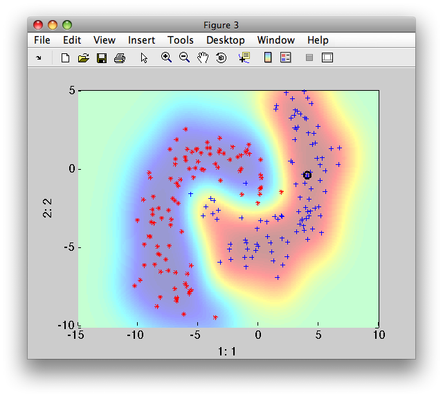
We can visualize the raw output of the pipeline action using sdscatter function:
>> sdscatter(b,p)
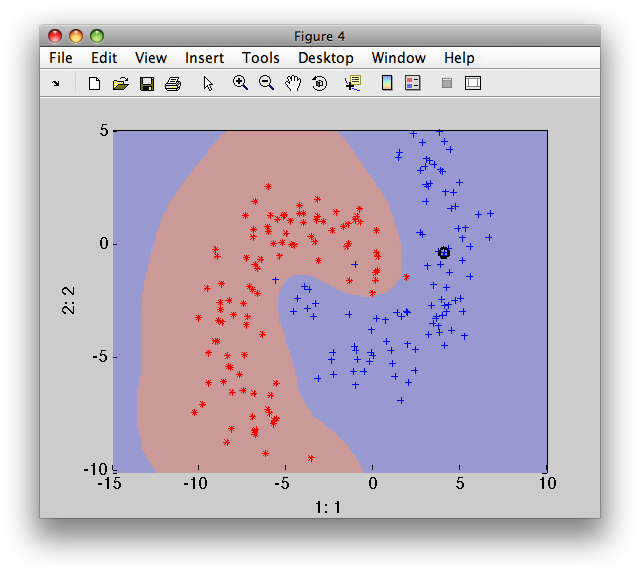
To provide decisions, we must add an operating point. We may use the
sddecide command that will add the default operating point thresholding
the SVM output at zero:
>> pd=sddecide(p)
sequential pipeline     2x1 'SVC+Decision'
 1  SVC                     2x1  (sdp_svc)
 2  Decision                1x1  thresholding on apple at op 1 (sdp_decide)

>> sdscatter(b,pd)
Finally, we will compare the execution speed of the trained SVC under libPRSD and LIBSVM. We create a random large dataset with 100 000 samples. We also need "labels" as the LIBSVM execution interface is designed for "testing", not only for "execution":
>> test=rand(100000,2);
>> lab=ones(size(test,1),1);

>> tic; [predict_label, accuracy, dec_values] = svmpredict(lab, test, model); toc
Accuracy = 0% (0/100000) (classification)
Elapsed time is 0.719287 seconds.

>> tic; out=test*p2; toc
Elapsed time is 0.309065 seconds.

>> 0.309065/0.719287
ans =
2.32
Execution under libPRSD gives us 2.32 times speedup.
The pipeline may be now exported using sdexport and directly run in a custom applications outside Matlab.