
- 14.1. Introduction
- 14.2. Confusion matrices
- 14.2.1. Normalized confusion matrices
- 14.2.2. Visualizing confusion matrix in a figure
- 14.2.3. Storing confusion matrices as strings
- 14.2.4. Rectangular confusion matrices
- 14.2.5. Confusion matrices for a set of operating points
- 14.2.6. Visualization of the per class errors
- 14.2.7. Cross-validation by rotation
- 14.2.8. How are the errors computed
- 14.2.9. Setting random seed
- 14.3. Accessing algorithms trained in cross-validation
- 14.4. Accessing per-fold data sets
- 14.5. Cross-validation by randomization
- 14.6. Leave-one-out evaluation
- 14.6.1. Leave-one-out over property
14.1. Introduction ↩
Design of pattern recognition system aims at providing two outcomes, namely the algorithm capable of performing decisions for new observations and the estimate of its performance. The classification performance may be reliable estimated only using the data unseen during training. In order to maximally leverage the limited amount of labeled examples available in most projects, perClass offers easy-to-use tools to perform sophisticated cross-validation strategies.
14.2. Confusion matrices ↩
Confusion matrix shows the match between true labels and classifier
decisions. It is a matrix with true labels on the rows and estimated labels
in the columns. The diagonals stores the number of correctly classified
objects, while the off-diagonal elements refer to the misclassified
objects. The example below shows the confusion matrix for a two class data
a where the labels are estimated using the trained classifier p:
>> truelab=a.lab;         %  sdlab object storing the labels
>> decisions=a*p;         %  sdlab object with classifier decisions
>> sdconfmat(truelab,decisions)
ans =

 True      | Decisions
 Labels    | apple  banana  | Totals
-------------------------------------
 apple     |   430     66   |   496
 banana    |    82    422   |   504
-------------------------------------
 Totals    |   512    488   |  1000
In the data a there are 496 apples, of which 66 are wrongly classified as
'banana', while 430 are correctly classified as 'apple'.
14.2.1. Normalized confusion matrices ↩
The confusion matrix can be normalized by the true number of objects per
class. The example below shows a confusion matrix for a eight class data
a where the labels are estimated using the trained pipeline p:
>> sdconfmat(truelab,decisions,'norm')

ans =

True      | Decisions
Labels    |       a       b       c       d       e       f       g       h  | Totals
---------------------------------------------------------------------------------------
a         |  0.916   0.080   0.000   0.000   0.000   0.003   0.000   0.000   | 1.00
b         |  0.019   0.953   0.000   0.000   0.000   0.000   0.029   0.000   | 1.00
c         |  0.000   0.000   0.917   0.083   0.000   0.000   0.000   0.000   | 1.00
d         |  0.000   0.000   0.242   0.758   0.000   0.000   0.000   0.000   | 1.00
e         |  0.000   0.000   0.000   0.000   0.979   0.021   0.000   0.000   | 1.00
f         |  0.000   0.000   0.000   0.000   0.023   0.976   0.000   0.000   | 1.00
g         |  0.000   0.006   0.000   0.000   0.000   0.000   0.958   0.036   | 1.00
h         |  0.000   0.000   0.000   0.000   0.000   0.000   0.034   0.966   | 1.00
---------------------------------------------------------------------------------------
14.2.2. Visualizing confusion matrix in a figure ↩
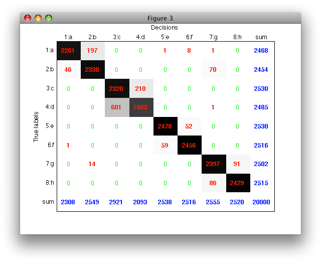
With 'figure' option, confusion matrix is visualized in a separate figure. Each matrix entry is rendered with a proportional gray-level allowing us to quickly spot the most important error patterns.
>> sdconfmat(a.lab,a*p,'figure')

ans =

3
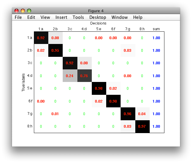
The row and column sums allow us to quickly compute useful error measures such as detection rates (dividing by the row sum) or precision (dividing by the column sum, i.e. number of samples assigned in a specific class).
Normalized matrix may be visualized in a figure using both the 'figure' and 'norm' options:
>> sdconfmat(a.lab,a*p,'figure','norm')

ans =

4
If an index (handle) of an existing figure is provided after the 'figure'
option, sdconfmat renders the confusion matrix into this figure instead
of opening a new one.
>> sdconfmat(a.lab,a*p,'figure',3,'norm')

ans =

3
14.2.3. Storing confusion matrices as strings ↩
With 'string' option, the confusion matrix can be saved as a string (str) and used for example to generate automatic reports:
>> str=sdconfmat(truelab,decisions,'string');

str =

 True      | Decisions
 Labels    |      a      b      c      d      e      f      g      h  | Totals
-------------------------------------------------------------------------------
 a         |  1119     99      0      0      0     13      1      1   |  1233
 b         |    25   1189      0      0      0      0     53      0   |  1267
 c         |     0      0   1114     95      0      0      0      0   |  1209
 d         |     0      0    306    962      0      0      1      0   |  1269
 e         |     0      0      0      0   1038    201      0      0   |  1239
 f         |     0      0      0      0    187   1033      0      0   |  1220
 g         |     0      5      0      0      0      0   1122    169   |  1296
 h         |     0      0      0      0      0      0    120   1147   |  1267
-------------------------------------------------------------------------------
 Totals    |  1144   1293   1420   1057   1225   1247   1297   1317   | 10000
When an output is requested and 'string' option is not used, a matrix is returned:
>> cm=sdconfmat(truelab,decisions);

cm =

  Columns 1 through 6

        1119          99           0           0           0          13
          25        1189           0           0           0           0
           0           0        1114          95           0           0
           0           0         306         962           0           0
           0           0           0           0        1038         201
           0           0           0           0         187        1033
           0           5           0           0           0           0
           0           0           0           0           0           0

  Columns 7 through 8

           1           1
          53           0
           0           0
           1           0
           0           0
           0           0
        1122         169
         120        1147
14.2.4. Rectangular confusion matrices ↩
sdconfmat can limit the set of classes or decisions to user specified
lists. Note that only subset of samples is used! Rectangular confusion
matrices arise in situations where we have 'outlier' true class but several
rejection decisions (e.g. 'background','not-fruit',...). In the example
below only the true labels of the classes a, c and d are visualized:
>> sdconfmat(truelab,decisions,'classes',{'a','c','d'})

ans =

 True      | Decisions
 Labels    |      a      c      d      e      f      g      h  | Totals
------------------------------------------------------------------------
 a         |   121      0      0      0      5      0      0   |   126
 c         |     0      0    109      0      0      0      0   |   109
 d         |     0     15    130      0      0      0      0   |   145
------------------------------------------------------------------------
 Totals    |   121     15    239      0      5      0      0   |   380
The classes and the decisions to be visualized can be chosen independently:
>> sdconfmat(truelab,decisions,'classes',{'a','c','d'},'decisions',{'a','b','c','d'})

ans =

 True      | Decisions
 Labels    |      a      b      c      d  | Totals
---------------------------------------------------
 a         |   121      0      0      0   |   121
 c         |     0      0      0    109   |   109
 d         |     0      0     15    130   |   145
---------------------------------------------------
 Totals    |   121      0     15    239   |   375
When no classes option is provided, the true label of all classes is
visualized as default:
>> sdconfmat(truelab,decisions,'decisions',{'a','b','c','d'})

ans =

True      | Decisions
 Labels    |      a      b      c      d  | Totals
---------------------------------------------------
 a         |   121      0      0      0   |   121
 b         |    57      0      0      0   |    57
 c         |     0      0      0    109   |   109
 d         |     0      0     15    130   |   145
 e         |     0      0      0      0   |     0
 f         |     0      0      0      0   |     0
 g         |     1      0      0      0   |     1
 h         |     0      0      0      0   |     0
---------------------------------------------------
 Totals    |   179      0     15    239   |   433
14.2.5. Confusion matrices for a set of operating points ↩
The confusion matrices from classifier soft output can be estimated for sets of operating points simultaneously. In this example, a test set with 10 000 samples is used and the confusion matrices are estimated at 10 000 randomly selected weighting-based operating points. The speed of the computation is also shown.
>> load eight_class     %  available in data subdir of perclass distribution
>> a
'Eight-class' 20000 by 2 sddata, 8 classes: [2468  2454  2530  2485  2530  2516  2502  2515]

>> [tr,ts]=randsubset(a,0.5)
'Eight-class' 9999 by 2 sddata, 8 classes: [1234  1227  1265  1242  1265  1258  1251  1257]
'Eight-class' 10001 by 2 sddata, 8 classes: [1234  1227  1265  1243  1265  1258  1251  1258]

>> p=sdquadratic(tr);
>> out=ts * -p;    %  get soft outputs

>> ops=sdops('w',rand(10000,8),tr.lab.list)
Weight-based operating set (10000 ops, 8 classes) at op 1

>> tic; [cm,ll]=sdconfmat(ops,out); toc
Elapsed time is 2.178765 seconds.

>> size(cm)

ans =

       8           8       10000
The variable cm stores a confusion matrix (which has size 8*8 for a eight
class problem) for each of the 10000 operating points. The sdconfmat
routine can also be used for a friendly visualization of a single confusion
matrix, e.g. the one at operating point number 42.
>> sdconfmat(cm(:,:,42),ts.lab.list)
True      | Decisions
Labels    |       a       b       c       d       e       f       g       h  | Totals
---------------------------------------------------------------------------------------
a         |   1171      45       0       0       0      16       2       0   |   1234
b         |    177     984       0       0       0       7      59       0   |   1227
c         |      0       0    1252      13       0       0       0       0   |   1265
d         |      0       0     476     767       0       0       0       0   |   1243
e         |      0       0       0       0    1095     170       0       0   |   1265
f         |      0       0       0       0     186    1072       0       0   |   1258
g         |      0       1       0       0       0       0     921     329   |   1251
h         |      0       0       0       0       0       0      37    1221   |   1258
---------------------------------------------------------------------------------------
Totals    |   1348    1030    1728     780    1281    1265    1019    1550   |  10001
14.2.6. Visualization of the per class errors ↩
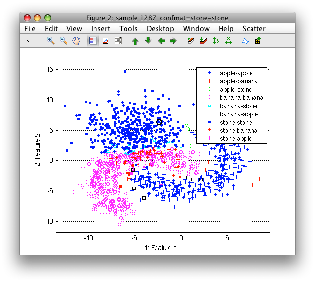
In order to inspect which samples are misclassified in a certain class it may be useful to visualize the errors of the confusion matrix. This can be achieved by creating a new sample property that combines the true labels with the decisions of the classifier.
>> load fruit_large
>> a
'Fruit set' 2000 by 2 sddata, 3 classes: 'apple'(667) 'banana'(667) 'stone'(666)

>> [tr,ts]=randsubset(a,200)
'Fruit set' 600 by 2 sddata, 3 classes: 'apple'(200) 'banana'(200) 'stone'(200)
'Fruit set' 1400 by 2 sddata, 3 classes: 'apple'(467) 'banana'(467) 'stone'(466)

>> p=sdmixture(tr)
[class 'apple' init:.......... 5 clusters EM:done  5 comp] [class 'banana' init:.......... 3 clusters EM:done  3 comp] [class 'stone' init:.......... 2 clusters EM:done  2 comp]
sequential pipeline       2x1 'Mixture of Gaussians+Decision'
 1 Mixture of Gaussians    2x3  10 components, full cov.mat.
 2 Decision                3x1  weighting, 3 classes

>> dec=ts*p
sdlab with 1400 entries, 3 groups: 'apple'(462) 'banana'(492) 'stone'(446)

>> ts.confmat=[ts.lab '-' dec]
'Fruit set' 1400 by 2 sddata, 3 classes: 'apple'(467) 'banana'(467) 'stone'(466)

>> ts'
'Fruit set' 1400 by 2 sddata, 3 classes: 'apple'(467) 'banana'(467) 'stone'(466)
sample props: 'lab'->'class' 'class'(L) 'ident'(N) 'confmat'(L)
feature props: 'featlab'->'featname' 'featname'(L)
data props:  'data'(N)

>> sdscatter(ts)
In the Scatter menu go to Use labels and select confmat.
14.2.7. Cross-validation by rotation ↩
Cross-validation is an evaluation strategy where the available design data set is split into several parts. One part is left out and the algorithm is trained on the remaining parts. The trained algorithm is executed on the part left out, and its decisions are used to compute the classification error. In perClass, this form of cross-validation is called 'rotation' because the definition of a test set rotates over parts and each sample is tested only once.
The cross-validation of a linear classifier is performed in as follows:
>> load fruit; a
'Fruit set' 260 by 2 sddata, 3 classes: 'apple'(100) 'banana'(100) 'stone'(60)
>> pd=sdgauss*sddecide
untrained pipeline 2 steps: sdgauss+sdp_decide
>> [s,res]=sdcrossval(pd,a)
10 folds: [1: ] [2: ] [3: ] [4: ] [5: ] [6: ] [7: ] [8: ] [9: ] [10: ]
s =

 10-fold rotation

 ind mean (std)  measure
   1 0.13 (0.02) mean error over classes, priors [0.3,0.3,0.3]

 average execution speed per fold: 0.74 msec

res =

      method: 'rotation'
       folds: 10
    measures: {'mean-error'}
        data: [10x1 double]
        mean: 0.1311
         std: 0.0160
   time_data: [10x1 double]
   time_mean: 7.3944e-04
    time_std: 6.1006e-06
   time_desc: [1x67 char]
The 10-fold cross-validation was performed using the default operating point weighting both classes equally (equal class priors). Note that the cross-validated algorithm must return decisions, not soft outputs.
The cross-validation result summary is provided as a string s. Detailed
results are given in the res structure. The res.data field stores the
per-fold estimates of performance measures. By default, the mean error over
classes with equal class priors is used. Additional measures may be
specified using the measures option:
>> sdcrossval(pd,a,'measures',{'class-errors','sensitivity','apple','specificity','apple'});
ans =

 10-fold rotation

 ind mean (std)  measure
   1 0.09 (0.03) error on apple
   2 0.11 (0.04) error on banana
   3 0.18 (0.05) error on stone
   4 0.91 (0.03) sensitivity on apple
   5 0.93 (0.02) specificity on apple

 average execution speed per fold: 0.75 msec
The 'class-errors' yields per-class error rates. Note that some measures, such as sensitivity or specificity require definition of the target class. For the list of the available performance measures see the ROC chapter.
We may wish to suppress the information displayed by sdcrossval. This may
be done either using the 'nodisplay' option or, globally, switching off all
display message of perClass commands using:
>> sd_display off
The number of cross-validation folds may be changed using the 'folds' option.
>> [s,res]=sdcrossval(pd,a,'folds',20);
>> res

res =

  method: 'rotation'
   folds: 20
measures: {'mean-error'}
    data: [20x1 double]
    mean: 0.1311
     std: 0.0167
   time_data: [10x1 double]
   time_mean: 7.3164e-04
    time_std: 2.9048e-06
   time_desc: [1x67 char]
Maximum number of folds in randomization method is limited by the number of samples in the smallest class.
14.2.8. How are the errors computed ↩
sdcrossval requires that each class in the test set maps to a classifier
decision. If a test set class does not have its counterpart in the list of
decisions, the corresponding error cannot be computed and sdcrossval
raises an error.
This may happen, for example, when training a detector. Lets assume a two-class problem with 'apple' and 'banana' classes.
>> b
'Fruit set' 1334 by 2 sddata, 2 classes: 'apple'(667) 'banana'(667)
We construct an untrained Gaussian detector on 'apple':
>> pd=sddetector([],'apple',sdgauss)
untrained pipeline 'sddetector'
Cross-validation on b throws an error message:
>> s=sdcrossval(pd,b)
10 folds: [1:   1: apple  -> apple
  2: banana -> non-apple
Warning: Some test set classes do not match to classifier decisions.
True classes ------------------------------
sdlist (2 entries)
 ind name
   1 apple
   2 banana
Decisions ------------------------------
sdlist (2 entries)
 ind name
   1 apple
   2 non-apple
??? Error using ==> sdroc.sdroc_err at 124
Cannot compute the error.
The error is raised because the trained detector has apple and
non-apple decisions while The banana class in the test set does not map
to any decision.
The solution is to make sure the detector's non-target class is called 'banana':
>> pd=sddetector([],'apple',sdgauss,'nontarget','banana','nodisplay')
untrained pipeline 'sddetector'
>> s=sdcrossval(pd,b)
10 folds: [1: ] [2: ] [3: ] [4: ] [5: ] [6: ] [7: ] [8: ] [9: ] [10: ]

s =

 10-fold rotation

 ind mean (std)  measure
   1 0.17 (0.01) mean error over classes, priors [0.5,0.5]
Note that the opposite situation is possible. Often, some of the classifier decisions do not map to any class present in the test set. Such situation appears, for example, in leave-one-out cross-validation where the single test object belongs to one class only or when evaluating classifiers with reject option.
14.2.9. Setting random seed ↩
For the sake of repeatability, we may fix the random seed:
>> [s,res]=sdcrossval(pd,a,'seed',42);
>> [s,res2]=sdcrossval(pd,a,'seed',42);
>> [res.data res2.data]

ans =

0.0556    0.0556
0.1444    0.1444
0.2222    0.2222
0.1000    0.1000
0.1444    0.1444
0.1222    0.1222
0.1333    0.1333
0.0889    0.0889
0.1000    0.1000
0.2000    0.2000
14.3. Accessing algorithms trained in cross-validation ↩
The optional third output of sdcrossval is an object that provides us
with access to algorithms trained in each fold.
>> [s,res,e]=sdcrossval(pd,a,'seed',42);
Here we access the pipeline trained in the second fold:
>> e(2)
sequential pipeline     2x1 'Gaussian model+Decision'
 1  Gaussian model          2x3  3 classes, 3 components (sdp_normal)
 2  Decision                3x1  weighting, 3 classes, 1 ops at op 1 (sdp_decide)
14.4. Accessing per-fold data sets ↩
The evaluation obeject e also allows us to access training or test set of
any fold.
>> [s,res,e]=sdcrossval(pd,a,'seed',42);
We need to provide it with the original data set used by sdcrossval and
with a fold index. To retrieve the training set, use the
gettrdata method:
>> tr=gettrdata(e,a,2)
'Fruit set' 234 by 2 sddata, 3 classes: 'apple'(90) 'banana'(90) 'stone'(54)
For a test set, use gettsdata method:
>> ts=gettsdata(e,a,2)
'Fruit set' 26 by 2 sddata, 3 classes: 'apple'(10) 'banana'(10) 'stone'(6)
Using these facilities, we may anytime investigate the confusion matrix of a given fold and compute any error or performance of interest:
>> sdconfmat(ts.lab,ts*e(2))

ans =

 True      | Decisions
 Labels    |  apple banana  stone  | Totals
--------------------------------------------
 apple     |    10      0      0   |    10
 banana    |     1      9      0   |    10
 stone     |     0      2      4   |     6
--------------------------------------------
 Totals    |    11     11      4   |    26

>> mean([0 1/10 2/6])   %  mean error over clases:

ans =

0.1444
14.5. Cross-validation by randomization ↩
perClass also provides 'randomization' type of cross-validation where training/test splits are constructed by random sampling of the total set.
By default, 50% of samples in each class is taken randomly in each fold.
>> [s,res]=sdcrossval(pd,a,'method','random');

>> res

res =

  method: 'randomization'
   folds: 10
measures: {'mean-error'}
    data: [10x1 double]
    mean: 0.1336
     std: 0.0110
Number of cross-valiadation folds in randomization is not limited.
Optional numerical argument of 'method','random' allows us to fix different
training fraction. Because it is passed directly to the
randsubset method, we may use it to:
- select a percentage of each class:
sdcrossval(pd,a,'method','random',0.8) - specify a number of samples per class:
sdcrossval(pd,a,'method','random',50) - select a training subset only from certain class/classes:
sdcrossval(pd,a,'method','random',[50 0])
The last option is useful when we want to cross-validate a detector trained in a one-class fashion (only on examples of a specific class).
>> a
'Fruit set' 260 by 2 sddata, 3 classes: 'apple'(100) 'banana'(100) 'stone'(60)

>> b=a(:,:,{'apple','banana'})
'Fruit set' 200 by 2 sddata, 2 classes: 'apple'(100) 'banana'(100)

>> pd2=sddetector([],'banana',sdgauss,'reject',0.1,'non-target','apple')
untrained pipeline 'sddetector'

>> [s,res,e]=sdcrossval(pd2,b,'method','random',[0 50]);

s =

 10-fold randomization

 ind mean (std)  measure
   1 0.14 (0.01) mean error over classes, priors [0.5,0.5]
Note that we specify the non-target name explicitly. If we did not do it,
the default non-target decision ('non-banana') would not match with any
true class and all non-target detections would be counted as errors. We
are also providing the vector parameter [0 50] of 'method','random' in the
order of classes in b.lab.list (banana is second).
>> e(1)
sequential pipeline     2x1 'Gaussian model+Decision'
 1  Gaussian model          2x1  one class, 1 component (sdp_normal)
 2  Decision                1x1  thresholding on banana at op 1 (sdp_decide)

>> tr=gettrdata(e,b,1) %  training data set does not contain apples
'Fruit set' 50 by 2 sddata, class: 'banana'

>> ts=gettsdata(e,b,1)
'Fruit set' 150 by 2 sddata, 2 classes: 'apple'(100) 'banana'(50)
14.6. Leave-one-out evaluation ↩
sdcrossval also supports the leave-one-out cross-valiation scheme where
each sample is once considered as a test set and training is performed on
remaining samples. Leave-one-out evaluation is beneficial for very small
sample sizes.
>> c=randsubset(a,[3 3 0])
'Fruit set' 6 by 2 sddata, 2 classes: 'apple'(3) 'banana'(3)

>> [s,res,e]=sdcrossval(sdlinear*sddecide,c,'method','loo')
6 folds: [1: ] [2: ] [3: ] [4: ] [5: ] [6: ]

s =

 6-fold leave-one-out

 ind mean (std)  measure
   1 0.33 (0.24) error on apple
   2 0.33 (0.24) error on banana

res =

  method: 'leave-one-out'
   folds: 6
measures: {'err(apple)'  'err(banana)'}
    data: [6x2 double]
    mean: [0.3333 0.3333]
     std: [0.2357 0.2357]

completed 6-fold evaluation 'sde_loo' (ppl: '')
By default, leave-one-out evaluation includes class error measures. Note that because each of our samples originates from one of the classes, the error on the other class is not defined.
>> res.data

ans =

 0   NaN
 0   NaN
 1   NaN
NaN     0
NaN     0
NaN     1
14.6.1. Leave-one-out over property ↩
Frequently used type of leave-one-out is cross-validation over specific labels, for example over patients or objects. This allows us to quickly valiate generalization error on unseen patient or object.
We may use the example small_medical data set that contains data samples originating from a medical diagnostic problem. For each sample, we know not only class and tissue type but also patient label.
>> load small_medical
>> a
'small medical' 300 by 10 sddata, 2 classes: 'disease'(57) 'no-disease'(243)

>> a'
'small medical' 300 by 10 sddata, 2 classes: 'disease'(57) 'no-disease'(243)
sample props: 'lab'->'class' 'class'(L) 'pixel'(N) 'patient'(L) 'tissue'(L)
feature props: 'featlab'->'featname' 'featname'(L)
data props:  'data'(N)
>> a.patient'
 ind name        size percentage
   1 Alex         122 (40.7%)
   2 Chris        121 (40.3%)
   3 Gabriel       57 (19.0%)
Using sdcrossval, we may quickly perform leave-one-patient-out validation:
>> pd=sdpca([],3)*sdlinear*sddecide
untrained pipeline 3 steps: sdpca+sdlinear+sdp_decide

>> [s,res]=sdcrossval(pd,a,'method','loo','over','patient')
3 folds: [1: ] [2: ] [3: ]

s =

 3-fold leave-one-out

 ind mean (std)  measure
   1 0.77 (0.15) error on disease
   2 0.22 (0.20) error on no-disease

res =

  method: 'leave-one-out'
   folds: 3
measures: {'err(disease)'  'err(no-disease)'  'mean-error'}
    data: [3x2 double]
    mean: [0.7745 0.2225]
     std: [0.1464 0.1981]